6.3.1. Identification task by the surface method

A velocity is denoted as x₂(t). Applying the model (6.1) the required parameters K_S and T_S can be calculated using the following relations:

K_s = lim x₂(t), t →∞

T_s = _K^K1 _s where K₁ = lim _∫ 0^t (K_s − x₂(λ))dλ,t →∞

The surface method is useful identification algorithm in the presence of disturbances. In this case the integral formula filtrates the measurement noises. Fig. 6.9 shows a typical application of this method to a DC servo identification problem.

6.3.2. Time domain identification experiment

In this experiment MSS includes the following modules: the DC motor with tachogenerator, inertia load, encoder module and gearbox module with the output disk. The magnetic break module can be added but in such a case the identified parameters of the system will be different.

To start the identification experiment type servo at the MATLAB prompt and Servo Control Window appears. Now, double click the Time domain identification button. The model shown in Fig. 6.10 opens.

Build model (in the case if it has not been done before). Next, select the Simulation/connect to target option and click the Simulation/Start real-time code. The servo starts to move and one can observe the velocities displayed in the screen (see Fig. 6.11).

Click the Calculate model button. This action starts the plot_ident.m file where the surface method is applied and parameters of the servo model are calculated. Next, Fig. 6.12 opens and two plots are displayed in the screen

• velocity obtained from the measurements (red),
• velocity calculated from the model (black).

On the top of the figure the calculated coefficients and mse corresponding to data fitting are displayed. The coefficients are also displayed in the Matlab command window.

0.05 Hz and sample time to 0.002.

• Build the model.

• Click the Simulation/connect to target and Start real-time code options to start

experiment. Next repeat the experiment for setting K_p = 0.0127 and K_p = 0.0254 .

The results of all experiments are given in Fig. 7.3 and Fig. 7.4. Note that oscillations of the system response appear if K_p = 0.0127 and K_p = 0.0254 .

Position control with P controller

80

60

40

20

0 -20 -40 -60 -80 0 5 10 15 20 25 30

Fig. 7.3 Response of the closed-loop system with P controller

	Kp=0.025	4
				Kp=0.0064
				Kp=0.0127

time [s]

Note, that the real system is nonlinear therefore the oscillations are damped very quickly. The controls shown in Fig. 7.4 do not reach zero. It is due to the dead zone of the system which can be observed at steady state characteristics given in Fig. 6.8 and is equal about +/

0.15. The non active controls belong to this range. Note, that the control saturates for K_p = 0.0254 .

Controls

1

0.8

0.6

0.4

0.2

0 -0.2 -0.4 -0.6 -0.8

-1

Fig. 7.4 Controls for different gains of the P controller

		Kp=	0.0064
			Kp=0.01	27
Kp	=0.0254

0 5 10 15 20 25 30 time [s]

In the table below steady state error is shown for the gain coefficients applied in these experiments. In accordance with theory if the K_p increases the steady state error decreases.

K	0.0064	0.0127	0.0254
∞ε	20 %	9.1 %	4.8 %

PD controller

The main goal of the controller tuning is to obtain the standard second order system step response. The general form of the second order transfer function is

_ω 2

G (s) = ^n ss² + 2ζω _ns +ω_n ²

If 0 <ζ < 1, then the step response of G_s (s) exhibits an exponentially damped sinusoidal character with the following features:

−ζπ  1−ζ

• percentage overshoot p_% = 100 e ²
• 2% settling time t_s = ⁴ ζω _n

π

• time to peak t_p =  ω_n 1−ζ ²

For given p_% and t_s one can calculate the damping coefficient ζ and natural frequency ω_n . Comparing a transfer function of the closed-loop system, which contains coefficients of controller, with the standard transfer function G_s (s) one can calculate the controller coefficients.

EXAMPLE

Assume that we want to design PD controller for the position control of the servo system as it is shown in Fig. 7.5: Note that at the first glance the state feedback controller is used. But

dα

remember that ω= . For this reason the applied controller is PD type.

dt

The requirements corresponding to the dynamics of the closed-loop system are as follows:

• settling time t_s ≤ 2.5[s]
• and maximal overshoot p_% ≤ 10

controller

servo

K

The servo system has the transfer function G(s) = ^s . The transfer function of the

s(T_ss +1) PD controller is K(s) = K_p + K_D s . The default values of the system coefficients are K_s = 186 [rad/s] and T_s= 1.04 [s].

Closing the control system we obtain the transfer function in the form

^K p^Ks

^Ts

G (s) = . ^z ₂ K_sK_D +1 K pKs

s + s + ^Ts ^Ts

Substituting values for the coefficients into the transfer function we obtain

7.2. PID Velocity control

The task of the velocity control is keep the desired velocity in present of the disturbances. The disturbances can be introduced as a change of the velocity reference signal or as change of the motor load. To disturb the reference velocity the potentiometer can be used. The load disturbances can be introduced by braking slightly the inertia load of the system. In the example the handy load disturbances were realized.

Click the Velocity control button in Servo Control Window and model shown in Fig. 7.17 opens.

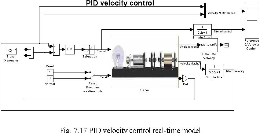
Set sine reference velocity, amplitude equal to 40 [rad/s] and frequency 0.1 [Hz] . Simulation time set 30 [s]. The Gain of the potentiometer set equal to zero. The coefficients of the PID controller set as K = 0.15 and K= 0.03 .

pi

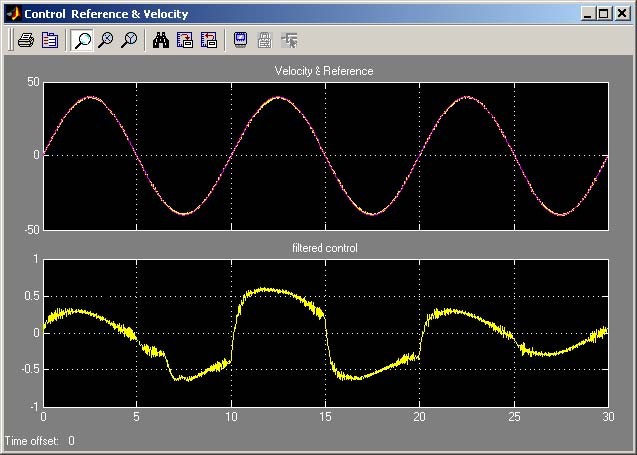
Build the model and run real time code. The results of the experiment are given in Fig.

7.18.

One can see that the disturbances of the motor load were introduced (by braking by hand the inertia load) at fifth second and finished at twentieth second. Note that the control increases in this time interval. The results are stored in VelCtrl variable placed in the Matlab workspace.

Type at the Matlab prompt :

plot(VelCtrl.time,VelCtrl.signals(1).values(:,2), r ,VelCtrl.time,VelCtrl .signals(1).values(:,1), k );grid;xlabel( time [s] );title( Reference velocity (red) -measured velocity (black) );

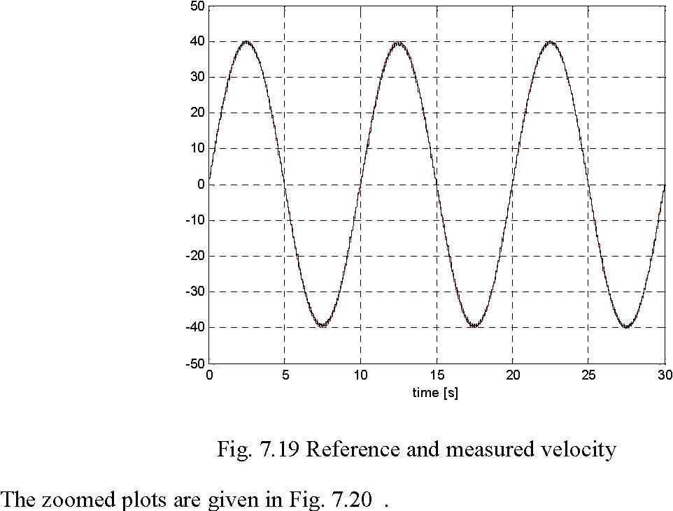
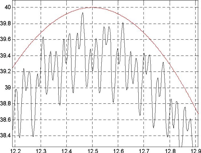
The plot is shown in Fig. 7.19 . In this scale the differences between the plots are unvisible. The details of the reference velocity and the measured velocity are shown in Fig. 7.20.

Reference velocity (red) -measured velocity (black)

time [s]

Reference velocity (red) -measured velocity (black)

time [s]

Fig. 7.20 Zoomed data

The tracking error of the velocity (at 12.5 second) is equal to 1%. Of course this error varies along the time axis but always is not large in relation to the error of the velocity measurements.

7.3. Multivariable control design

The section demonstrates how properties of a closed-loop system are influenced by the design parameters: the closed-loop roots and sampling period. Two methods of the closed-loop systems design are shown. The first is based on pole placement and is applied for continuous systems. The second control method, known as "deadbeat control" is used for discrete systems.

7.3.1. Pole-placement method

A closed-loop system with feedback gains from the states is analysed. The approach we wish to apply is a pole placement. It means that we can change the closed-loop system roots. There are different ways of achieving this. One of the design methods is described below.

The continuous-time system is represented by the state equation:

x& = Ax + Bu

y = Cx

The state controller realises a linear feedback control law in the form: u = K( y_d − y),

where K is a feedback gain matrix and y_d is the desired output vector.

We request that the roots of the closed system are equal to λ₁,λ₂ (fixed). The design methods consist in finding K that the roots of the closed-loop system are in the desired locations. That means, we assume dynamic properties of the closed system. It can be shown that there exists a linear feedback that gives a closed-loop system with roots specified if and only if the pair (A, B) is controllable. It is clear that closed-loop system has to be stable and it is a sine qua non assumption of the design.

The state matrix of the closed-loop system is

A_c = (A − BKC ).

For the case of the DC motor the matrix A_cis given as



01 Kk 1+ Kk

s 1 s



 ⎢

 ⎥

A_c =

−

−

2

,

^Ts ^Ts

and the characteristics equation has the form 1+ Kk Kk

2 s 2 s 1

λ + λ += 0.

^Ts ^Ts

By means of the feedback gains, the location of roots of the characteristics equation may be changed. From the Vieta s formula we obtain

Kk 1+ Kk

s 1 s 2

λ ⋅ λ = (λ + λ ) =− ,

12 12

^Ts ^Ts and we can calculate k₁ and k₂ from

λ ⋅ λ ⋅T_s (λ + ₂)T_s +

1 2 1 ^λ 1

k₁ = k₂ =− . (7.1)

^Ks ^Ks

It is clear that we can require a desired behaviour of the closed-loop system but we have to keep the control between appropriate limits |u(t)| ≤ 1. When the control variable saturates, it is necessary to be sure that the system behaves properly.

EXAMPLE

Assume we want to design a closed-loop system without oscillations. A possible selection of the roots is:

λ₁ =−2 and λ₂ =−3.

For the identified parameters (an example) K_s = 186 [rad/s] and T_s= 1.04 [s] we can

calculate k₁, k₂ from formula (7.1)

₁ = 0.0335 and k = 0.0226

^k 2

Then, we simulate the closed-loop system with feedback gains k₁, k₂.

Perform the following steps:

• type K=[0.0335 0.0226] and servo at the MATLAB prompt.
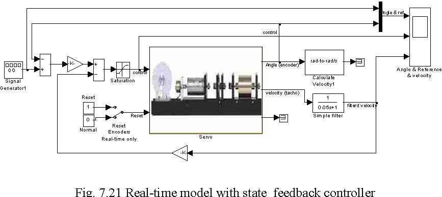
• Double click the State feedback control continuous and State feedback controller buttons. The model shown in Fig. 7.21 opens. Assuming a desired range of change of the output disk position equal to pi/8 set reference input signal equal to 100*pi/8 (it is the measured angle at the input to the gearbox). Also set frequency of the reference input to

0.1 Hz and sample time to 0.002.

• Build the model.
• Click the Simulation/connect to target and Start real-time code options to start the experiment.

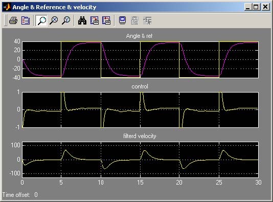
The results are presented in Fig. 7.22. Notice, that the response of the system is slow and not

accurate. The reference angle is reached with accuracy equal to 6% and the settling time is

about 4[s].

We can change the roots of the closed-loop system to make the system faster. Assuming λ₁ =−4 and λ₂ =−5 we obtain: k₁ = 0.1118 and k₂ = 0.0449 .

State feedback controller

Type at Matlab prompt K=[0.0335 0.0226] and repeat the experiment with the new values of k . The experimental results are shown in Fig. 7.23. Notice that the response of the

1^, k2

system is faster and more accurate. The reference angle is reached with accuracy equal to 2.3% and the settling time is 2.5 [s]. These results outperform the previous one.

In both experiments the control saturates despite that the goals of the design are achieved.

 ⎥⎦

7.3.2. Deadbeat controller

It is the control method unique to discrete systems in which we calculate feedback gains in such a way that roots of the closed system are equal to zero. This control strategy has the property that it drives the states of a closed-loop system from an arbitrary values to zero in at most N steps (dim(A)=N). It is the fastest possible discrete controller.

The sampling time T0 is the only design parameter. The magnitude of the control variable u can be decreased by increasing the sampling time T0, or vice versa. For a given range of the reference variable step a suitable sample time can be determined. The main problem of the design is the saturation of system actuators.

The discrete system is described by a discrete state equation:

x[( n + 1)T ] = Ax[nT ] + Bu[nT ]

0 D 0 D 0

y[nT ] = Cx[nT ].

0 D 0

The matrices A_Dand B_D are calculated from the continuous state-space model using the following, well known, relations:

dt B

T

0





AT0 At

∫

C_D C^AD

=I.

B

 ⎢

=

=

=

e e

D

0

For a discrete model of the DC motor matrices A_dand B_d have the form

Modular Servo System -User’s Manual

T

0

T

0









−−

TsTs

− _S −

−

K

S

(T

(1

))

1 _S (1

)

  ⎢

T

  ⎥

  ⎢

T

  ⎥

e

e^AD

=

e

AT

0

=

0

,

B

D

=

.

T

0

T

0

−

−

Ts

Ts

(1 −

e

)

0

e

K

S

If we assume reachability of the pair ( A_D,B_D ) and a control law in the form u[( n)T ] = K( y [nT ] − y[nT ])

0 d 00

K = [k₁k₂], we obtain the closed-loop system shown in Fig. 7.24.

y [nT₀]

y_d [nT₀]

x[( n +1)T ] = Ax[nT ] + Bu[nT ]

 u 0 d 0 d 0

y[nT ] = Cx[nT ]

0 d 0

Fig. 7.24. Closed-loop system with the feedback gain

The closed-loop system is described by the equation

x[( n +1)T ] = (A − B KC )x[nT ] + B Ky [nT ].

0 D DD 0 Dd 0

Feedback gains for the deadbeat controller are calculated from the equation:

det( λI − (A_D − B_DKC _D )) |_{λi =0,i=1,2} = 0.

Design method

We can design deadbeat controller using a simulation method. The following steps are necessary in this case:

1. choose the sampling time T₀,
2. create a discrete model,
3. calculate feedback gains,
4. simulate the closed-loop discrete system,
5. if the control overruns saturation limits increase the sampling time T₀and repeat the steps from 1 to 5.

EXAMPLE

This example shows how to design the deadbeat controller.

A goal of the control is to track a reference signal (the angle of the motor shaft). The reference signal is assumed a square wave.

Type servo at the MATLAB prompt and then double click the State feedback control discrete button. To design the controller click the Calculate deadbeat controller button. It executes the servo_calc_db.m file where a coefficients of deadbeat controller are calculated according to algorithm shown above. The body of this file is listed below. Notice the comments in the file.

% Continuous linear model of the servo system. % Parameters of the servo are read from workspace

A=[0 1;0 -1/Ts]; B=[0; Ks/Ts]; C = [1 0;0 1]; D = zeros( 2, 1 );

% If the distance to the reference signal is big control value in the % first sample time is big too. Due to we are looking for such a T0 % when control does not saturate,we must assume the maximum change of % the reference signal.

delta_ref=[25*pi;0]; && it is maximal change of the reference signal

% we start look for T0 T0=0.1; for i = 1:200 T0=T0+0.005;

% ** Discrete model for sampling time T0*

[Ad,Bd]=c2d(A,B, T0);

% Now we calculate a coeffitients of deadbeat controller % using the formula : eig(Ad-Bd*K)=0

Z=[Bd(1) Bd(2); Ad(2,2)*Bd(1)-Ad(1,2)*Bd(2) Ad(1,1)*Bd(2)]; X=[Ad(1,1)+Ad(2,2);Ad(1,1)*Ad(2,2)]; K=(Z\X) ;

% Now coefficients of the controller are saved in K

% checking if the control saturates in the first sample time: % u(1)=K*delta_ref;

if abs(K*delta_ref)<=1 K T0 && write K and T0 in Matlab command window return end end

The variables K and T₀are stored in the MATLAB workspace after the execution of the

above m-file. In our case for K_s = 186 [rad/s] and T_s= 1.04 [s] we obtain

K = [0.0127 0.0091] and T₀ = 0.7950 . Now double click the State feedback controller buttons to perform the real-time experiment and the model depicted in Fig. 7.25 opens.

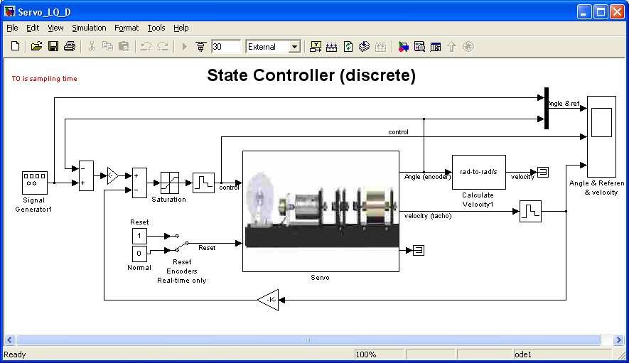
This model differs in details from the other models. Due to the fact that the model is discrete, and the sampling time T₀can vary from experiment to experiment T₀is read from

the Matlab workspace. Variable T₀is located in the Simulink model in the following places: in Fixed step size in tag Solver which is located in Simulation/Simulation Parameters option, in all Zero-Order Hold blocks and in the mask of the Servo device driver. There is no filter connected to the output of the tachogenerator. The filter applied in other models is not discrete one and can not be used here. However it is interesting how the controller works without filtering of the velocity signal.

Set the amplitude of the input signal to 100*pi/8 (as in the previous example), the frequency of reference signal to 0.05 Hz. Set simulation time equal to 60 [s] and time range in the scope also 60 [s]

Due to the fact that the model includes variables K and T₀and some settings was changed rebuild it. Click Simulation/connect to target. Click the Start real-time code option to start the experiment. The results are shown in Fig. 7.26.

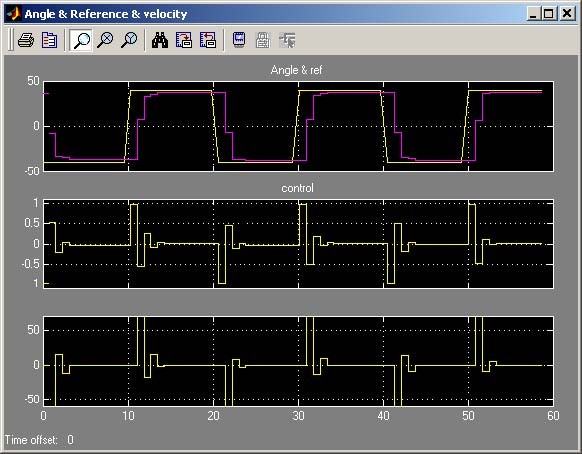
Note, that the system does not reach the reference angle in two steps. In fact, the servo is a nonlinear system and it is only approximated by a linear model. Notice that this control is significant only during two first sample intervals.

7.4. Optimal design method: LQ controller

The linear-quadratic problem (LQ problem) is a central one in the theory and applications of optimal control. There are two versions of the LQ problem: the open-loop and the closed-loop optimal control problems. Either the optimal control is given as an explicit function of time for fixed initial conditions, or the optimal controller is synthesised. Further only the second case is considered. The main result of the finite-dimensional linear-quadratic theory is that under suitable assumptions the optimal feedback controller is linear with respect to the state, and constant with respect to time.

The synthesis of the discrete and continuous LQ controller is presented below. For a very small value of the sampling time the response of the discrete system converges to the response of the corresponding continuous system. The most important question for a designer of a control system, as far as LQ control problem is concerned, is how to select the weighting factors in the cost function.

Let us examine separately the continuous and discrete LQ problems.

7.4.1. The continuous case

The dynamical model of the DC-motor is described by the linear differential equations:

x& = Ax + Bu

y = Cx ,

where the matrices A, B and C have the form

⎡01 ⎤ 0  ⎡10⎤

A =  ¹ ⎥, B =  ^Ks ⎥, C = . (7.2)

0 − ⎢01⎥

 ⎥⎢⎥⎣⎦

TT

 S ⎦ S 

The desired input time history of the state vector is given by y (t) = [ y (t), y (t)] .

d 1d 2d

Hence, the error vector e is defined

e(t) = y_d (t) − y(t).

A typical quadratic cost function (performance index) has the form

Tk

J (u) = ¹_2 ∫[e^T (t)Qe (t) + u^T (t)Ru (t)] dt ,

0

where:

• matrix Q ≥ 0, Q is a nonnegative definite matrix,
• matrix R > 0, R is a positive definite matrix,
• the (A,B) pair is controllable.

The weighting matrices Q and R are selected by a designer but they must satisfy the above conditions. It is most easily accomplished by picking the matrix Q to be diagonal with all diagonal elements positive or zero. Some positive weight (|R|≠0) must be selected for the control, otherwise the solution will include infinite control gains.

The values of elements of Q and R matrices weakly correspond to the performance specification. A certain amount of trial and error is required with a simulation program to achieve satisfactory result. A few guidelines can be recommended. For example, if all states are to be kept under close regulation and Q are diagonal with entries so selected that a fixed percentage change of each variable makes an equal contribution to the cost. The matrix R is also diagonal.

If the maximum deviations of the servomechanism outputs are: , and the

^y1max ^y2 max

maximum deviation of control is u_max , then the cost is:

2 22

Q( 1,1)y ₁ + Q( 2,2 )y ₂ + Ru

The coefficients of the Q and R matrices can be set related to the rule: 1 11

Q(1,1) = ₂, Q(2,2) = ₂ and R = ₂

( y )( y )(u )

1max 2max max

This rule can be modified to satisfy desired root locations and transient response for selected values of weights. One must avoid saturation effects both of outputs and control.

Due to the differences in methods of analysis, problem formulation and the form of results, we strongly distinguish the linear-quadratic problem with a finite settling time from that with a infinite settling time. However in applications we frequently encounter the situation when the termination moment of the control process is so far away that it does not affect the current control actions. The infinite-time optimal control problem is then posed. The cost function is replaced by the formula:

∞

J (u) = _∫[e^T (t)Qe (t) + u^T (t)Ru (t)] dt (7.3)

0

Then the optimal scalar control u ^* and the optimal trajectory vector y ^*are given

u ^* = K( y_d − y ^*) ^(7.4)

where K is the feedback matrix.

The optimal control problem is now defined as follows: find the gain K such that the feedback law (7.4) minimises the cost function (7.3) subject to the state equation (7.2). The calculation of the control variable which minimizes the criterion (7.3) is a dynamic optimisation problem. This problem can be solved by variation calculus applying the maximum principle due to the Bellman optimisation principle. The procedure returns the optimal feedback matrix K, the matrix S, the unique positive definite solution to the associated matrix Riccati equation:

SA + A^TS -SBR^-1B^TS + Q = 0

Due to the quadratic appearance of S, there is more than one solution, and S must be positive definite to select the correct one. The procedure returns also the matrix E, the closed-loop roots:

E = eig(A -B*K*C)

The vector K can be calculated by a numeric iterative formula on the basis of the Riccati equation. The associated closed-loop system e& = (A − BKC )e is asymptotically stable.

To solve the LQ controller problem the lqry function from the Control System Toolbox can be used. The synopsis of lqry is: [K,S,E] = lqry(A,B,C,D,Q,R).

In this case the matrix of weights Q relate the outputs y instead of the state x. For the servomechanism D is the row matrix with two zero elements. The function lqry computes the equivalent Q, R and calls lqr,

The control u is not constrained. This assumption can not be satisfied for a real physical system. One must remember that if the control u saturates then it not satisfies the LQ problem. To return to the LQ problem the amplitude of the u signal should be diminished. In such a case a designer tunes the relative weights between state and control variables. To perform that the simulation tools are recommended.

EXAMPLE

The goal of the control is to track a reference signal which is defined as a square wave. Set the amplitude of the reference input signal equal to 100*pi/8. Set the frequency of the reference input to 0.1 Hz and sample time to 0.002 [s].

Type servo at the MATLAB prompt and then double click the State feedback control continuous button. To design LQ controller click the Calculate LQ controller button. It executes servo_calc_lq.m file presented below:

% State space representation of servo: A=[0 1;0 -1/Ts]; B=[0; Ks/Ts]; C = [1 0;0 1]; D = zeros( 2, 1 );

% Set Q and R matrices. These values can be changed by a user Q=[50 0;0 1]; R=1000;

% calculate coefficients of the LQ controller [K,S,lambda]=lqry(A,B,C,D,Q,R);

% type K in Matlab command window K

For the default values: K_s = 186 [rad/s] and T_s= 1.04 [s] we obtain K = [0.2236 0.054] .

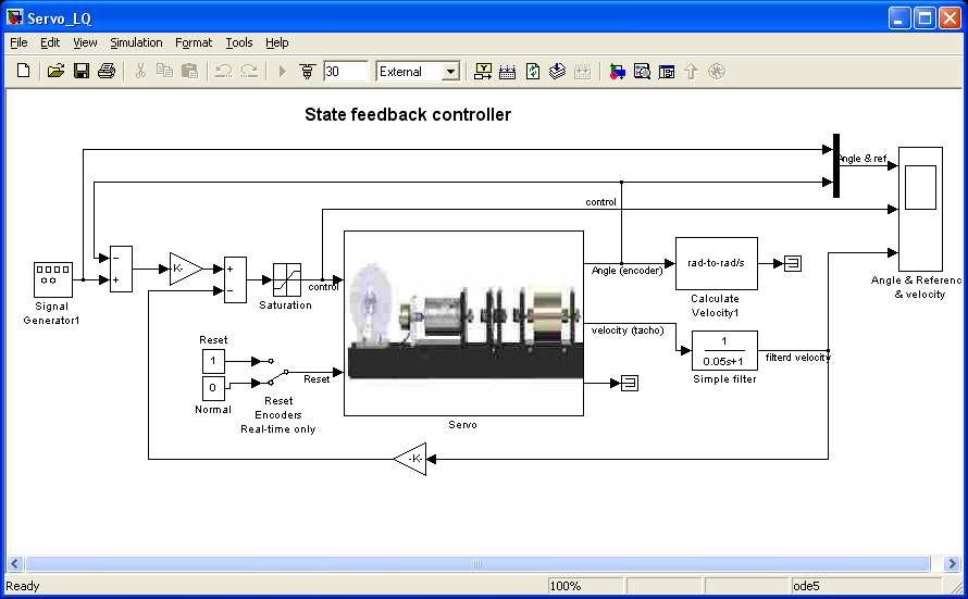
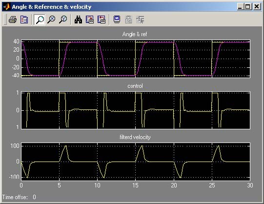
To perform the real-time experiment click the State feedback controller button. When the model opens (see Fig. 7.27), check parameters of the reference signal. Build the model, click Simulation/connect to targetand Start real-time code option to start experiment. The results are given in Fig. 7.28. Notice that the reference signal is reached with accuracy equal to 0.58% and without overshoots. The control signal saturates.

7.4.2. The discrete case

If we introduce the sampling period T₀then the model can be discretized. The discrete model of the DC motor has the form:

x[( n + 1)T ] = Ax[nT ] + Bu[nT ]

0 D 0 D 0

(7.5)

y[nT ] = Cx[nT ].

0 D 0

where the matrices: A_D, B_D and C_D are in the form

T

0

T

0









−−

TsTs

− _S −

−

K

S

(T

(1

))

1 _S (1

)

  ⎢

T

  ⎥

  ⎢

T

  ⎥

ee

^AD

=

e

AT

0

=

0

,

B

D

=

.

T

0

T

0

−−

TsTs

(1 −

e

)

0

e

K

S

The matrix A_Dis the fundamental solution of the differential equation (7.5) calculated for the sampling period T₀. The explicit values of the matrices A_Dand B_D of the servo system can be obtained numerically by the use ofc2d function. C2d converts a continuous state representation to the discrete corresponding to the continuous. The procedure is a part of Control System Toolbox. One must simply type the command:

[ A_D,B_D ]=c2d(A,B, T0)

The optimal feedback law:

u[nT ] = Ke [nT ], e[nT ] = y − y[nT ]

0 00 d 0

minimizes the cost function:

N

J (u)

=

∑

[

e

^T (n)Q(n)e(n) u^T (n)Ru (n)] (7.6)

+

n=0

subject to the state equation (7.5). The dlqry function from the Control System Toolbox is used to solve the discrete-time linear-quadratic control problem. The synopsis of the dlqry and lqry programs are identical. The dlqr also solves and returns matrix S, the unique positive definite solution to the associated discrete iterative matrix Riccati equation:

TT T −1 T

S = ASA − A SB (R + B SB ) B SA + Q .

i+1 DiD DiD DiD DiD

The feedback matrix is derived from S by

T − T

K = (R + B SB )¹ B SA

DD DD

EXAMPLE

A goal of the control is the same as in the continuous case example. Assume that sampling time for discrete system T₀ = 0.1[s].

In Servo Control Window double click the State feedback control discrete button. To design the LQ controller click the Calculate LQ controller button. It executes the servo_calc_lq_d.m file presented below.

% State space representation of servo: A=[0 1;0 -1/Ts]; B=[0; Ks/Ts]; C = [1 0;0 1]; D = zeros( 2, 1 );

% set sampling time T0=0.1; % calculate discrete model from continuous [Ad,Bd]=c2d(A,B, T0)

% set Q and R matrices Q=[50 0;0 1]; R=1000;

% design discrete LQ controller

[K,S,lambda]=dlqry(Ad,Bd,C,D,Q,R); K

For the default values: K_s = 186 [rad/s] and T_s= 1.04 [s] we obtain K = [0.139 0.0395] .

To perform the real-time experiment click the State feedback controller button and the model shown in Fig. 7.25 opens. It is the same model as are previously applied to deadbeat control. Set the frequency of the reference signal to 0.1 [Hz] the simulation time to 30 [s] and the time range of the scope to 30 [s]. These settings correspond to the values which have been assumed for the continuous LQ controller. Build model, click theSimulation/connect to target and the Start real-time code options to start experiment.

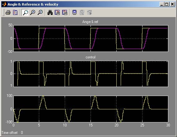
The results are shown in Fig. 7.28. They are similar to these for the continuous controller. The reference signal is reached with accuracy equal to 1% and without overshoots. The control signal saturates as in the previous example.

8. Description of the Modular Servo class properties

The CServo is a MATLAB class, which gives the access to all the features of the RT-DAC4/PCI board supported with the logic for the MSS model. The RT-DAC4/PCI board is an interface between the control software executed by a PC computer and the power-interface electronic of the modular servo model. The logic on the board contains the following blocks:

• incremental encoder registers – two 32-bit registers to measure the position of the incremental encoders. There are two identical encoder inputs, that may be applied to measure the shaft positions of two modular servo blocks;
• incremental encoder reset logic. The incremental encoders generate different output waves when the encoder rotates clockwise and counter-clockwise. The encoders are not able to detect the reference (“zero”) position. To determine the “zero” position the incremental encoder registers have to be set to zero by the computer program;
• PWM generation block – generates the Pulse-Width Modulation output signal. Simultaneously the direction signal and the brake signal are generated to control the power interface module. The PWM prescaler determines the frequency of the PWM wave;
• power interface thermal flags –the thermal flags can be used to disable the operation of the overheated DC motor;
• interface to the on-board analog-to-digital converter. The A/D converter is applied to measure the position of the external potentiometer and to measure the output voltage of the tachogenerator.

All the parameters and measured variables from the RT-DAC4/PCI board are accessible by

appropriate properties of the CServo class. In the MATLAB environment the object of the CServo class is created by the command: object_name = CServo; The get method is called to read a value of the property of the object: property_value = get( object_name, ‘property_name’ ); The set method is called to set new value of the given property: set( object_name, ‘property_name’, new_property_value ); The displaymethod is applied to display the property values when the object_name is entered in the MATLAB command window.

This section describes all the properties of the CServo class. The description consists of the following fields:

Purpose	Provides short description of the property
Synopsis	Shows the format of the method calls
Description	Describes what the property does and the restrictions subjected to the property
Arguments	Describes arguments of the set method
See	Refers to other related properties
Examples	Provides examples how the property can be used

8.1. BaseAddress

Purpose: Read the base address of the RT-DAC4/PCI board.

Synopsis: BaseAddress = get( sv, ‘BaseAddress’ );

Description: The base address of RT-DAC4/PCI board is determined by computer. Each CServo object has to know the base address of the board. When a CServo object is created the base address is detected automatically. The detection procedure detects the base address of the first RT-DAC4/PCI board plugged into the PCI slots.

Example: Create the CServo object:

sv = CServo;

Display their properties by typing the command:

sv

Type: CSERVO Object BaseAddress: 54272 / D400 Hex Bitstream ver.: x402 Encoder: [ 0 46606 ][bit] Reset Encoder: [ 0 0 ] Input voltage: [ 0.1123 0.1123 ][V] PWM: [0] PWM Prescaler: [ 0 ] Thermal status: [ 0 ] Thermal flag: [ 1 ] Angle: [ 0 71.4927 ][rad] Time: 31.657 [sec]

Read the base address: BA = get( sv, ‘BaseAddress’ );

8.2. BitstreamVersion

Purpose: Read the version of the logic stored in the RT-DAC4/PCI board.

Synopsis: Version = get( sv, ‘BitstreamVersion’ );

Description: The property determines the version of the logic design of the RT-DAC4/PCI board. The modular servo models may vary and the detection of the logic design version makes it possible to check if the logic design is compatible with the physical model.

8.3. Encoder

Purpose: Read the incremental encoder registers.

Synopsis: enc = get( sv, ‘Encoder’ );

Description: The property returns two digits. They are equal to the number of impulses generated by the corresponding encoders. The encoder counters are 32-bit numbers so the values of this property is from (–2³¹) to (2³¹-1). When an encoder counter is reset the value is set to zero. The incremental encoders generate 4096 pulses per rotation. The values of the Encoder property should be converted into physical units.

See: ResetEncoder, Angle, AngleScaleCoeff

8.4. Angle

Purpose: Read the angle of the encoders.

Synopsis: angle_rad = get( sv, ‘Angle’ );

Description: The property returns two angles of the corresponding encoders. To calculate the angle the encoder counters are multiplied by the values defined as the AngleScaleCoeff property. The angles are expressed in radians.

See: Encoder, AngleScaleCoeff

8.5. AngleScaleCoeff

Purpose: Read the coefficients applied to convert the encoder counter values into physical units.

Synopsis: scale_coeff = get( sv, ‘AngleScaleCoeff’ );

Description: The property returns two digits. They are equal to the coefficients applied to convert encoder impulses into radians. The incremental encoders generate 4096 pulses per rotation so the coefficients are equal to 2*pi/4096.

See: Encoder, Angle

8.6. PWM

Purpose: Set the direction and duty cycle of the PWM wave.

Synopsis: PWM = get( sv, ‘PWM’ ); set( sv, ‘PWM’, NewPWM );

Description: The property determines the duty cycle and direction of the PWM wave. The PWM wave and the direction signals are used to control the DC drive so in fact this property is responsible for the DC motor control signal. The NewPWM variable is a scalars in the range from –1 to 1. The value of –1, 0.0 and +1 mean respectively: the maximum control in a given direction, zero control and the maximum control in the opposite direction to that defined by –1.

The PWM wave is not generated if the thermal flag is set and the power amplifier is overheated.

See: PWMPrescaler, Therm, ThermFlag

Example: set( sv, ‘PWM’, [ -0.3 ] );

8.7. PWMPrescaler

Purpose: Determine the frequency of the PWM wave.

Synopsis: Prescaler = get( sv, ‘PWMPrescaler’ ); set( sv, ‘PWMPrescaler’, NewPrescaler );

Description: The prescaler value can vary from 0 to 63. The 0 value generates the maximal PWM frequency. The value 63 generates the minimal frequency. The frequency of the generated PWM wave is given by the formula:

PWMfrequency = 40MHz / 1023 / (Prescaler+1)

See: PWM

8.8. Stop

Purpose: Sets the control signal to zero.

Synopsis: set( sv, ‘Stop’ );

Description: This property can be called only by the set method. It sets the zero control of the DC motor and is equivalent to the set(sv, ‘PWM’, 0) call.

See: PWM

8.9. ResetEncoder

Purpose: Reset the encoder counters.

Synopsis: set( sv, ‘ResetEncoder’, ResetFlags );

Description: The property is used to reset the encoder registers. The ResetFlags is a 1x2 vector. Each element of this vector is responsible for one encoder register. If the element is equal to 1 the appropriate register is set to zero. If the element is equal to 0 the appropriate register counts encoder impulses.

See: Encoder

Example: To reset only the first encoder register execute the command: set( sv, ‘ResetEncoder’, [ 1 0 ] );

8.10. Voltage

Purpose: Read two voltage values.

Synopsis: Volt = get( sv, ‘Voltage’ );

Description: Returns the voltage of two analog inputs. Usually the analog inputs are applied to measure the position of the external potentiometer and the output of the tachogenerator.

8.11. Therm

Purpose: Read thermal status flag of the power amplifier. Synopsis: Therm = get( sv, ‘Therm’ ); Description: Returns the thermal flag of the power amplifier. When the temperature of a

power amplifier is too high the flag is set to 1.

See: ThermFlag

8.12. ThermFlag

Purpose: Control an automatic power down of the power amplifiers.

Synopsis: ThermFlag = get( sv, ‘ThermFlag’ ); set( sv, ‘ThermFlag’, NewThermFlag );

Description: If the ThermFlag or NewThermFlag are equal to 1 the DC motor is not excited by the PWM wave when the power interface is overheated.

See: Therm

8.13. Time

Purpose: Return time information.

Synopsis: T = get( sv, ‘Time’ );

Description: The CServo object contains the time counter. When a CServo object is created the time counter is set to zero. Each reference to the Time property updates its value. The value is equal to the number of milliseconds which elapsed since the object was created.

8.14. Quick reference table

Property name	Operation*	Description
BaseAddress	R	Read the base address of the RT-DAC4/PCI board
BitstreamVersion	R	Read the version of the logic design for the RT-DAC4/PCI board
Encoder	R	Read the incremental encoder registers
Angle	R	Read the angles of the encoders
AngleScaleCoeff	R	Read the coefficient applied to convert encoder positions into radians
PWM	R+S	Read/set the parameters of the PWM waves
PWMPrescaler	R+S	Read/set the frequency of the PWM waves
Stop	S	Set the control signal to zero
ResetEncoder	R+S	Reset the encoder counters or read the reset flags
Voltage	R	Read the input voltages
Therm	R	Read the thermal flags of the power amplifiers
ThermFlag	R+S	Read/set the automatic power down flag of the power amplifier
Time	R	Read time information

• R – read-only property, S – allowed only set operation, R+S –property may be read and set

8.15. CServo Example

To familiarise a reader with the CServo class this section presents an M-file example that uses the properties of the CServo class to measure the static characteristics of the DC motor (see section 6). The static characteristics is a diagram showing the relation between DC motor control signal and the motor shaft velocity. The M-file changes the control signal and waits until the MSS reaches steady-state. The velocity of the shaft is obtained in two ways:

• the M-file measures the output voltage from the tachogenerator,
• the M-file measures the encoder position in two time points and calculates the velocity as the difference of positions divided by the time period between the time points.

The M-file is written in the M-function form. The name of the M-function is Servo_PWM2RPM.

The function requires two parameters:

• CtrlDirection -a string that selects how to change the control value. The A string causes the control is changed in ascending manner (from -1 to 1), the D string causes the control is changed in descending order (from 1 to -1) and the R string causes reverse double changes (from -1 to +1 and after that from +1 to -1),
• MinControl, MaxControl – minimal and maximal control signal values. The control signal changes within the region defined by these values,
• NoOfPoints -number of characteristics points within the MinControl/MaxControl range. The exact number of points of the characteristics declared by this parameter is enlarged to two points namely: MinControland MaxControl.

The body of this function is given below. The comments within the function describe the main stages.

function ChStat = Servo_PWM2RPM( … CtrlDirection, MinControl, MaxControl, NoOfPoints )

CtrlDirection = lower( CtrlDirection ); NoOfPoints = max( 1, NoOfPoints+1 );

% Calculate control step Step = (MaxControl-MinControl) / NoOfPoints;

switch CtrlDirection case a  Ctrl = MinControl:Step:MaxControl; case d  Ctrl = MaxControl:-Step:MinControl; case r  Ctrl = [ MinControl:Step:MaxControl MaxControl:-Step:MinControl]; otherwise % This should not happen error( The CtrlDirection must be A , D or R . ) end

FigNum = figure( Visible , on , ...  NumberTitle , off , ...  Name , Velocity vs. PWM characteristic , ...  Menubar , none );

sv = cservo; Control = []; VelEnc = []; % Optionally set the PWM prescaler %set( sv, pwmprescaler , 20);

for i=1:length(Ctrl)

% Set a new control value

set( sv, PWM , Ctrl(i) );

% Reset encoders

set( sv, ResetEncoder , [1 1] );

set( sv, ResetEncoder , [0 0] );

pause( 5 )

AuxEnc = get( sv, Encoder ); TimeBeg=gettime;

pause( 2 )

% Calculate velocity based on the encoder positions

VelEnc(i,:) = 2*pi*(get( sv, Encoder )-AuxEnc)/ …

4096/((gettime-TimeBeg)/1000); % [rad/s]

Control(i) = get( sv, PWM );

Volt(i,:) = get( sv, Voltage );

% Perform 10000 A/D conversions and calculate average values

AuxVolt = [0 0];

for j=1:10000

AuxVolt = AuxVolt + get( sv, Voltage );

end

Volt(i,:) = AuxVolt/10000;

% Convert voltage into velocity

Volt2Vel = 20.4*Volt(:,2);

% Plot data

subplot(211);

plot( Control, VelEnc(:,2), Control, VelEnc(:,2), x ); grid

title( Encoder velocity vs. PWM );

xlabel( PWM control value ); ylabel( Velocity [rad/s] );

subplot(212);

plot( Control, Volt2Vel, Control, Volt2Vel, x ); grid

title( Tacho velocity vs. PWM );

xlabel( PWM control value ); ylabel( Tacho velocity [rad/s] ); end % Assign data to the structure returned by the function ChStat.Control = Control;ChStat.TachoVelocity = VelEnc(:,2); ChStat.EncoderVelocity = Volt2Vel;

% Switch off the control set( sv, Stop );

The diagrams generated by the call

servo_pwm2rpm( r ,-0.5,0.5,19),

are shown below. The diagrams present the velocity of the shaft as function of the control signal. The control signal changes from –0.5 to +0.5. The velocity value is obtained in two ways. At the upper diagram the velocity is calculated from the encoder positions. The lower diagram presents the velocity obtained from the tachogenerator.

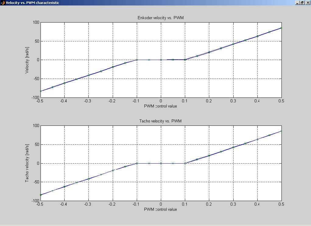
The values on the diagram may vary from experiment to experiment as they depend on the configuration of the modular servo set-up.

9. Some technical data

Fig. 9.1 Dimensions and weights of the MSS mechanical elements

15	Φ 20 68 Φ 66	Φ 25 5 5 Φ 66 8,5	Φ 20
	Brass inertia load 2.030 kg	0.055 kg Aluminium wheels	0.05 kg

Data sheet of the DC motor

is available at

http://www.buehlermotor.com/cgi-bin/sr.exe/productpageus&productpage=54

The gearbox ratio N = 100