2. Starting, testing and stopping procedures
2.1. Starting procedure
Assemble the external USB board, Control Interface and Tower Crane together. Invoke MATLAB and type:
Tcr
The USB_TCrane_Main window opens (see Fig.2.4). The pushbuttons indicate an action that executes callback routines when the user selects a menu item.
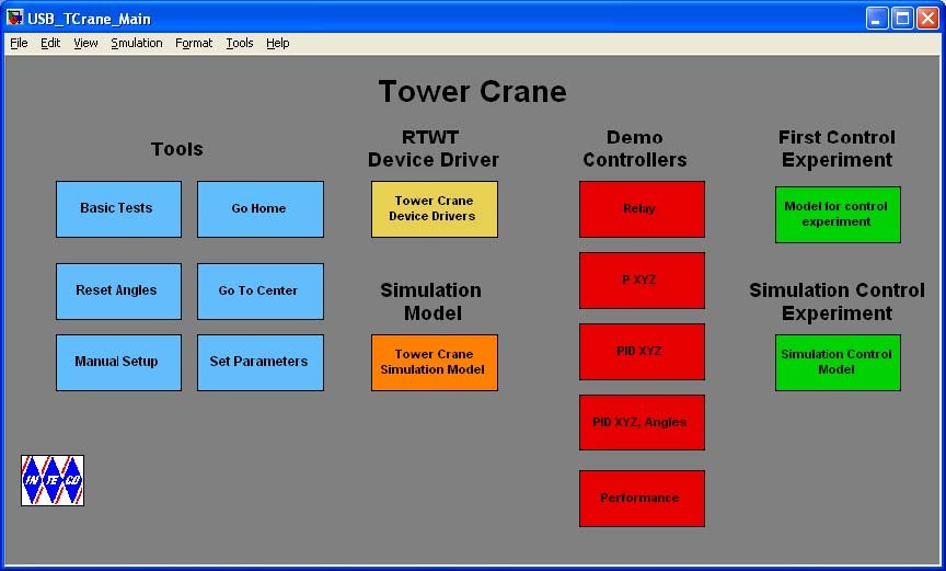
Fig.2.4 The USB_TCrane_Main window
The window contains testing tools, drivers, models and demo applications. You can see a number of pushbuttons ready to use.
 In the case if the RT-DAC/USB I/O board is used only one software module can communicate with USB board. Remember do not open more than one
Simulink model at time.
2.2. Testing and troubleshooting
This section explains how to perform the tests. These tests enable to check the correctness of the mechanical assembling and wiring. The tests have to be performed obligatorily after assembling the system. They are also necessary in a case of an incorrect operation of the system. The tests can be helpful to find an eventual reason of the system fail. The tests have been designed to validate the existence and sequence of measurements and controls. They do not relate to accuracy of the signals.
The operational space of the tower crane is illustrated in Fig. 2.5.

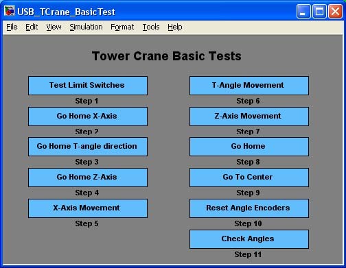
First, you have to be aware that all signals are transferred in a proper way. Eleven checking steps are applied.
• Double click the Basic Tests button. The following window appears (Fig. 2.6):
The first step is to check the proper operation of the limit switches. There are three switches applied to stop the system motions and to secure the system against destruction if the cart or the arm approach the limits. The z axis motion switch is a typical mechanical one, two other switches are contactless activeted if a metalic object comes closer to the switch.
• Double click the Test limit switches button. The window presented in Fig. 2.7 opens:
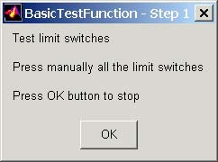
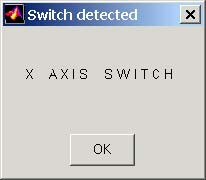
Turn on manually one by one all switches related to x, and z directions. The z-axis switch turn on by your finger. The contactless switches turn on putting a coin close to the switches. When a switch is turned on one can hear a sound signal. If one turns on the x-axis limit switch then the window shown in Fig. 2.8 appears. It means that the switch operates properly. Close the window – click the OK button. When an arbitrary switch is not detected please check cables corresponding to the undetected switch.
Next, you can check if the cart, arm and payload move in the right direction and if the system stops at the desired limit position. The system is moved in the chosen direction until it reaches the zero position (at this point the switch limit must be active).
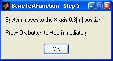
• Double click the Go Home X-axis (T-angle direction and Z-axis) button and observe the behaviour of the system. The window (Fig. 2.9) opens. You can interrupt the motion clicking the OK button.

After performing tests along three directions the system is stopped at the zero position. The encoders of the x, and z directions are automatically reset to zero value.
If motion in a given direction is not observed check the cables and plugs related to this direction.
The next three steps perform the change of the system position from the initial position to the initial + 0.3 [m] or 0.3 rad position along a selected direction.
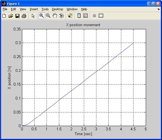
Click the OK button the plot of the movement is displayed (Fig. 2.13)

Now you must set the load motionless and click Yes. The angle encoders are reset and the zero position is memorised by the system.
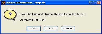
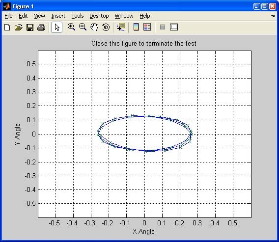
• To check if the angles are correct double clicks the Check Angles button. The window shown in Fig. 2.15 opens. Then manually move the load to a non-zero position and release it. Click the OK button. Observe the motion at the screen (Fig. 2.16)
2.3. Stopping procedure
The system is equipped with the hardware stop pushbutton. It cuts off the transfer of control signals to the crane. The pushbutton does not terminate the real-time process running in the background. Therefore to stop the task you have to use Simulation/Stop from the pull-down menu in the model window.
3. Main Control Window
The user has a rapid access to all basic functions of the Tower Crane control system from USB_TCrane_Main. It includes tests, drivers, models and application examples.
USB_TCrane_Main shown in Fig.2.4 contains four groups of the menu items:
-
Tools
-
Drivers
-
Demo Controllers
-
Experiments
3.1. Tools
The respective buttons in the TOOLS column perform the following tasks:
Basic Tests - checks the measurements and control.
Go Home – moves the crane to the zero position, resets the encoders and sets control signals to zero. This button is frequently used before starting an experiment. When the Go Home procedure is finished we can be sure that the values of all measured signals have been set to zero.
Reset Angles – resets the angle measuring encoders in a fixed position. If you stop the payload manually, perform the Reset Angles operation to be sure that the payload angles measured by the encoders show zeros.
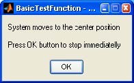
Go to Center -moves the crane to the center of the crane operational space and switches off the control. Remember that the zero position of the crane is in the point where: the x position and the angle are equal zero. Most experiments cannot be started from the zero point. Go to Center enables the crane quickly move to the center.
Set Parameters -enables the user to change the default values of Rail limits, Base Address and z displacement. The default value of the Base Address may cause a conflict with other devices installed in the computer. One has to be ensured that his computer configuration is free from address conflicts.
The user can also need to adjust the crane operational space dimensions to his requirements. Fig. 3.17 presents the window where such changes can be done. The user has to type numerical values into the editable text boxes.

All introduced modifications are written to the configuration file. Please be ☞ careful with introducing them. Writing the rail limit values exceeding the real rail limits may result in damage of the system elements.
Manual Setup – The Tower Crane Manual Setup program gives access to the basic parameters of the laboratory 3-dimensional setup. The most important data transferred from the RT-DAC/USB board and the measurements of the crane signals as well as status signals and flags may be shown. Moreover the control signals of three DC drives may be set.
Double click the Manual Setup button and the screen shown in Fig. 3.18 opens.
The application contains five frames:
-
The RT-DAC/USB board frame presents the main parameters of the USB board.
-
The Control frame allows to change the control signals.
-
The x, and z positions are given in the X, and Z positions frame.
-
The X and Y angles frame contains the angle measurements.
-
The Status and flags frame displays state of the status signals and flag values.
All the data presented in the Tower Crane Manual Setup program are updated 20 times per second.
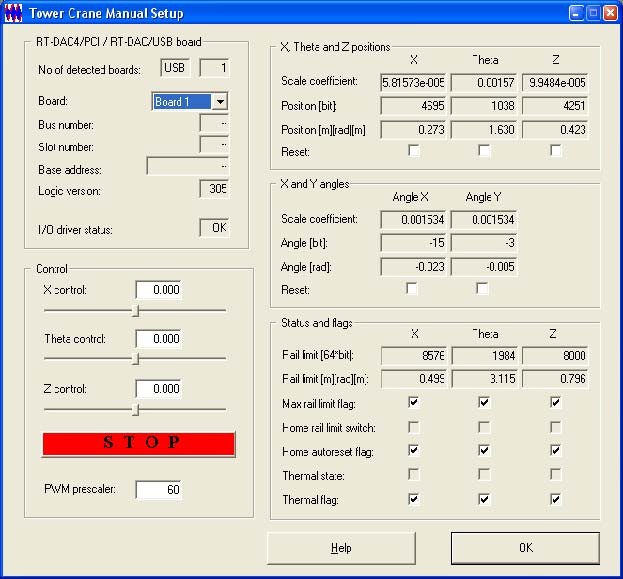
RT-DAC/PCI / RT-DAC/USB board
The frame contains the parameters of the RT-DAC/PCI or RT-DAC/USB boards detected by the computer. With respect to the interface board applied to control the system the program operates with RT-DAC/PCI or RT-DAC/USB boards.
No of detected boards
The number of detected RT-DAC boards. If the number is equal to zero it means that the software has not detect any board. When more then one board is detected theBoard list must be used to select the board that communicates with the program.
Board
The list applied to select the board currently used by the program. The list contains a single entry for each RT-DAC/PCI or RT-DAC/USB board installed in the computer. A new selection executed at the list automatically changes values of the remaining parameters within the frame. If more then one RT-DAC/USB board is detected the selection at the list must point to the board applied to control the tower crane system. Otherwise the program is not able to operate in a proper way.
Bus number
The number of the PCI bus where the current RT-DAC/PCI board is plugged-in. The parameter may be useful to distinguish boards, when more then one board is used and the computer system contains more then a single PCI bus. This parameter is only active if the RT-DAC/PCI boards are applied.
Slot number
The number of the PCI slot where the current RT-DAC/PCI board is plugged-in. The parameter may be useful to distinguish boards, when more then one board is used. This parameter is only active if the RT-DAC/PCI boards are applied.
Base address
The base address of the current RT-DAC/PCI board. The RT-DAC/PCI board occupies 256 bytes of the I/O address space of the microprocessor. The base address is equal to the beginning of the occupied I/O range. The I/O space is assigned to the board by the computer system and may be different among computers. This parameter is only active if the RT-DAC/PCI boards are applied. The base address is given in the decimal and hexadecimal forms.
Logic version
The number of the configuration logic of the on-board FPGA chip. A logic version corresponds to the configuration of the RT-DAC board defined by this logic and depends on the version of the tower crane model.
I/O driver status
The status of the driver that allows the access to the I/O address space of the microprocessor. The status has to be OK string. In other case the twer crane software HAS TO BE REINSTALLED.
Control
The frame enables to set the control signals of three DC drives.
X control, control, Z control The control signals of the X, and Z DC drives may be set by entering a new value into the corresponding edit field or by dragging the corresponding slider. The control values may vary from –1.0 to +1.0. The value of –1, 0.0 and +1 mean respectively: the maximum control in a given direction, zero control and the maximum control in the opposite direction to that defined by –1. If a new control value is entered in an edit field the corresponding slider changes respectively its position. If a slider is moved the value in the corresponding edit field changes as well.
S T O P
The pushbutton is applied to switch off all the control signals. When pressed all the control values are set to zero.
PWM prescaler
The control signals are generated as PWM waves. The PWM prescaler sets the divider of the PWM reference signal. The frequency of the PWM controls is equal to:
FPWM = 20000/1023/(1+PWMPrescalerr) [kHz]
This parameter sets the frequency of all PWM control signals. The parameter may vary from 0 to 63. It causes the changes of the frequency of the PWM control signals from 19.55kHz to 305Hz.
X, and Z positions
The frame presents data related to the X, and Z axis positions. The X position is the arm position. The position relates to the angle position of the crane arm with the cart. The position of the load is denoted as Z. All position measurements are performed by the incremental encoders. There are the following four fields associated with each axis.
Scale coefficient
The value applied to calculate the position expressed in meters or radians. The value read from the encoder counter is multiplied by the corresponding scale coefficient to obtain the position in meters or radians.
Position [bit]
The value read from the corresponding encoder counter.
Position [m]
The position expressed in meters. The value read from the encoder counter is multiplied by the corresponding scale coefficient to obtain the position in meters.
Position [rad]
The position expressed in radians. The value read from the encoder counter is multiplied by the corresponding scale coefficient to obtain the position in radians.
Reset
The checkbox applied to reset the corresponding encoder counter. If the box is checked the related position is set to zero. The box has to be unchecked to allow position measurements. As the incremental encoders are not able to detect an origin position the origin of the system has to be set by limit switches (see the description of the Home autoreset flag) or has to be set in a programming manner by a user. The Reset checkboxes are applied to set the origin position (zero position) in a programming way.
X and Y angles
The frame presents data related to the X axis angles of the load. The angle measurements are performed by the incremental encoders. There are the following four fields associated with each angle.
Angle X and angle Y denote the angle deviations in X and perpendicular to X
☞ direction, respectively. They are denoted by α and β in the mathematical model (see Fig. 6.63).
Scale coefficient
The value applied to calculate the angle expressed in radians. The value read from the encoder counter is multiplied by the corresponding scale coefficient to obtain the angle in radians.
Angle [bit]
The value read from the corresponding encoder counter.
Angle [rad]
The angle expressed in radians. The value read from the encoder counter is multiplied by the corresponding scale coefficient to obtain the position in radians.
Reset
The checkbox applied to reset the corresponding encoder counter. If the box is checked the related angle is set to zero. The box has to be unchecked to allow angle measurements. As the incremental encoders are not able to detect an origin position the origin of the system has to be set in programming manner by a user. The angle reset checkboxes should be checked when the load remains motionless in the downright position.
Status and flags
The frame presents status data and flags related to the X, and Z directions. There are seven fields associated with each directions.
Position limit [64*bit]
The board is able to automatically turn off the control signal if the tower crane system is going outside the operating range. The field defines the maximum value of the corresponding encoder determining the maximum accessible position. If the encoder reaches this position the board is able to stop the generation of the DC control signals moving the system outside the operating range.
Position limit [m] or [rad]
The field defines the maximum accessible position expressed in meters or radians. If the system reaches this position the board is able to stop the generation of the DC control signals moving the system outside the operating range. The maximum position expressed in meters or angle position expressed in radians is obtained as the result of the multiplication of 64, maximum position expressed in bits and the corresponding scale coefficient.
Max position limit flag
If the checkbox is selected the board turns off the control when the system is going to move outside the operating range. It is recommended to keep this checkboxes selected all the time.
Home position limit switch
The boxes that present the state of the home limit switches. If a limit switch is pressed the corresponding box is selected.
Home autoreset flag
The flag that causes automatic reset of the encoder counter when the corresponding home limit switch is pressed. If the checkbox is unchecked (the flag is inactive) the state of the limit switch does not influence the state of the encoder counter.
Therm state
The signal that presents the state of the thermal flag of the power interface. The system contains three power amplifiers for the DC drives. If the power amplifier is overheated the corresponding box is checked.
Therm flag
The flag that causes to turn off the control if the power amplifier is overheated. If the flag is unchecked, the power amplifier is overheated and the temperature increases the amplifier itself turns off the control signal. It is recommended to keep this checkboxes selected all the time.
Click the Go to Center button and open next Manual Setup button. You will see the
changes of measured positions. Note that the X position, angle position and Z position
have changed their values and become the center positions in the crane workspace.
3.2. Drivers
The main driver is located in the RT Device Driver column. The driver is a software go-between for the real crane MATLAB environment and the RT-DAC/USB board. This driver is dedicated to the control and measurement signals. Click the Tower Crane Device Drivers button and the driver window opens (Fig. 3.19)
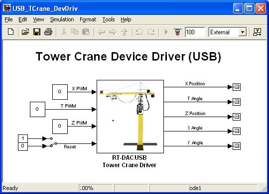
The driver has three PWM inputs (DC motor controls) for the X and Z-axes and T-angle direction. There are 10 outputs of the driver: X position, T position, Z position, two angles (see section 8) and additionally three safety switches. According to a pre-programmed logic the internal XILINX program of the RT-DAC/USB board can use the switches to stop the DC motors.
When one wants to build his own application one can copy this driver to a new model.
 Do not make any changes inside the original driver. They can be made only inside its copy!!!
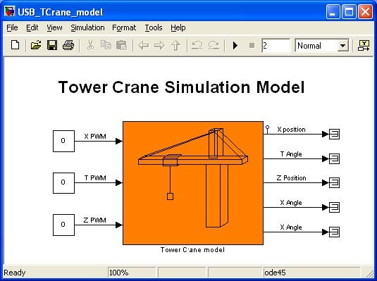
Simulation Model – the simulation model of the crane is located under this button. Its signal environment is identical as the model given in the Tower Crane Device Drivers except the lack of the safety switches (see Fig. 3.20). These switches are not used in the simulation mode. The simulation model is used for many purposes: identification, controllers design, etc.
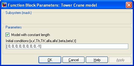
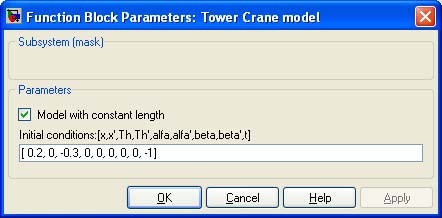
In the mask shown in Fig. 3.21 one can introduce initial values for the model state variables. Additionally, by marking the checkbox you can use the model with constant length (see section 8 for details).

 Set solver options to: Fixed step and Fixed-step size equal to 0.001 atmost. A greater value results in errors.
The C source code of the modeltc.c file is attached to the DevDriv directory.
3.3. Demo Controllers
A number of control algorithms are given. These demos can be used to familiarise the user with the crane system operation and enable to create the user-defined control systems. The examples must be rebuilt before using. Due to similarity of the examples we focus our attention only on one of them.
Click the Relay button the model appears (see Fig. 3.22):
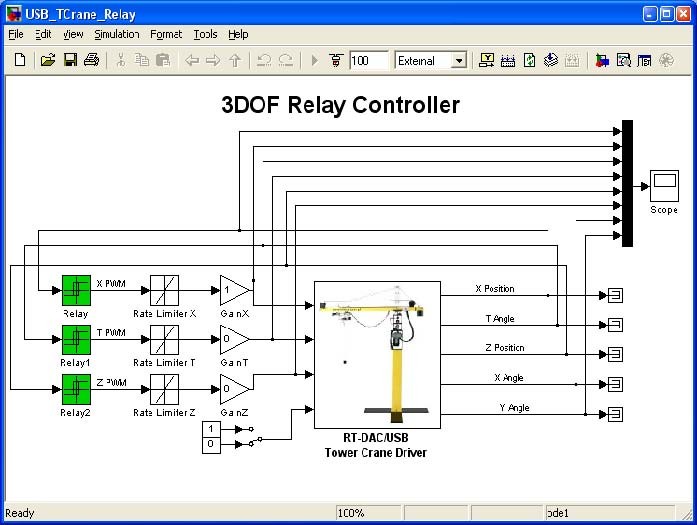
Notice that the model looks like a typical Simulink model. The device driver is applied in the same way as other blocks from the Simulink library. The only difference is that the model is used by RT-CON to create the executable library, which runs in the real-time mode.
The goal of the model is the relay control in the x-axis only. Therefore GainY and GainZ are set to zero.
-
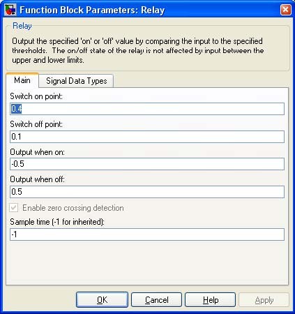
Look at the mask of the Relay block connected to the X PWM input (Fig. 3.23).
-
Note that the control generated by the controller has two values: +0.5 and –0.5. The On/Off limits are 0.2 and 0.6. This means that the crane will move between these limits with the speed corresponding to the control value equal to 0.5.
-
To choose the starting point inside the [−0.5, 0.5] range go to the USB_TCrane_Main window and click the Go to Center button.
-
Then, choose the Tools pull-down menus in the Simulink model window. The pop-up menus provide a choice between predefined items. Choose the RTW Build item. A successful compilation and linking process is finished with the following message:
Model TowerCrane_Relay.rtd successfully created ### Successful completion of Real-Time Workshop build procedure for model: TowerCrane_Relay
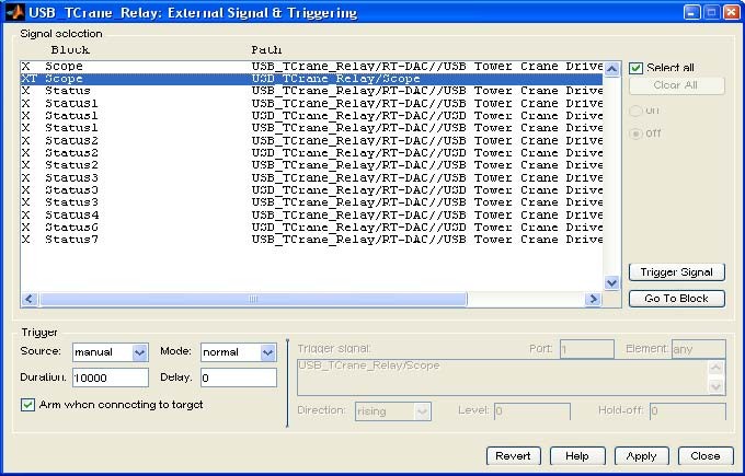
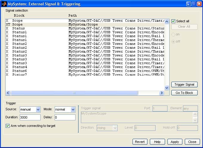
If any error occurs then the message corresponding to the error is displayed in the MATLAB command window. Next, click the Tools/External Mode Control Panel item and next click the Signal Triggering button. The window shown in Fig. 3.24 opens.
-
Select XT Scope , set Source as the manual option, mark the Arm when connect to Target option and close the window.
-
Return to the model window and click the Simulation/Connect to Target option. Next,
-
Observe the plots in the scope and click Stop Simulation after some time. Results of the example are shown in Fig. 3.25.
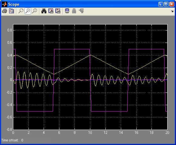
The X position starts from 0.38 and changes between 0.4 and 0.1. The control (magenta line) is a square wave in the range [−0.5, 0.5]. The control is switched when the limit values are reched by the X position. Note that the X angle in the form of a sinusoidal curve is modulated by the control interacting with friction.
4. Your first real-time control experiment
We recommend two experiments. In the first one only the control loop in the x direction is defined. In this case stabilisation of the angle of the payload is neglected. In the second experiment the stabilisation of the payload angle is added.
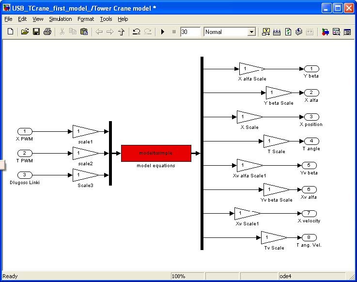
We begin from a simple real-time control experiment. A PID controller for the x position of the cart is built. The USB_TCrane_first model is given in Fig. 4.26. To invoke it, click Model for control experiment button in the The USB_TCrane_Main window. In this case, the active control corresponding to the x cart position is all you need. The Simulink blocks included in the control are drawn with dropped shadows to distinguish active control loops from disabled loops. In our first experiment we use the X position of the cart PID controller with its P control part activated only.

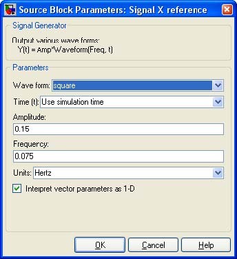
We define a source of a desired x position signal as the X reference/Generator from the Simulink library (see Fig. 4.27)
As usual, at the begining the GO HOME and GO TO CENTER actions are performed. The proper experiment starts in the middle of the x, y rails. Therefore the constant block shift is required.
Next, we define the signals to be used. These are X-reference – the desired x position value, X-position, X-control and X-angle. These signals, among others, are connected to the Scope block.
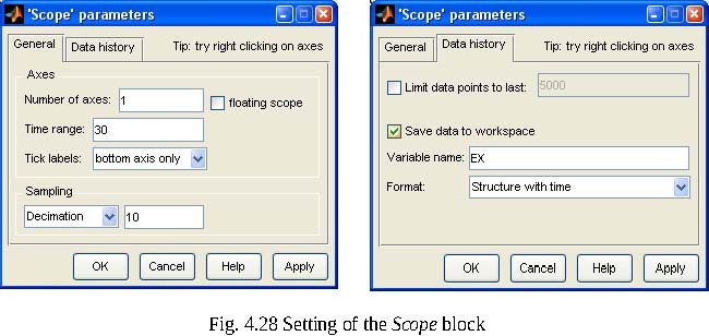
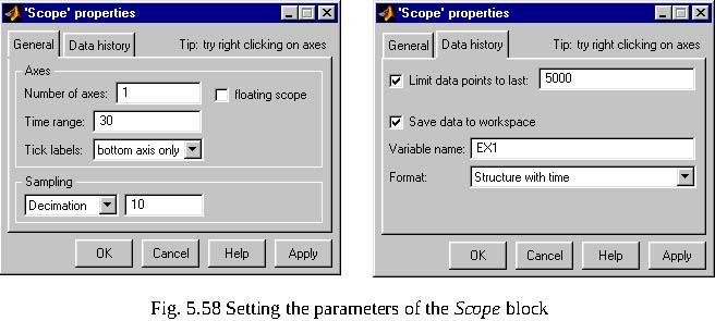
The properties of this block are defined below (see Fig. 4.28). This window opens after the selection of the Scope/Properties tab. Mark the Save data to workspacecheckbox, define the Variable name as EX1 and the data format as structure. This means the collected data within 30 seconds time range are saved to the workspace in the structure EX1. The sampling period set in the Simulation Parameters window (see Fig. 4.28) is equal to 0.01, Sampling Decimation is set to 10. Therefore, the size of EX1 is equal to: 30 s / (0.01 s × 10) + 1= 301
Next, return to USB_TCrane_first and select the Simulation/Parameters item. In the Solver tab select Fixed Step and set Stop time equal to 30. The Real-time Workshop options must be defined as in Fig. 4.29.

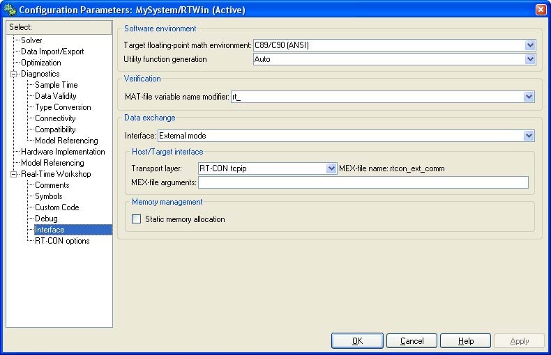
Next connection with external mode and transport layer has to be set. Interface page, responsible for connection with external target system, is shown in Fig. 4.30.To fulfil it properly a user must select External mode in Interface edit window. After that the user have to set RT-CON tcpip in the Transport layer edit window.

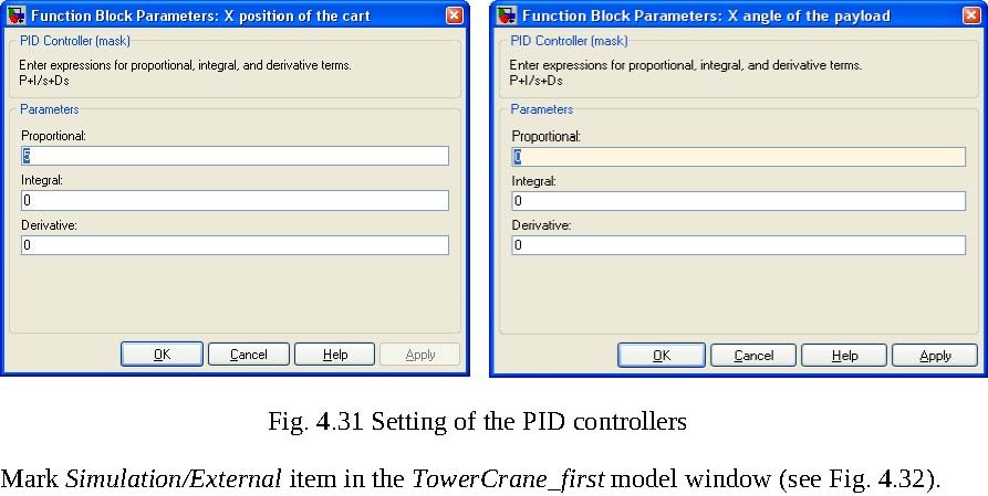
Set the PID controllers. We set the Proportional part of the X position of the cart PID controller as indicated by the arrow in Fig. 4.31. The X angle of the payload PID controller remains inactive. The other controlling loops are disabled due to the Gain blocks set to zero (see Fig. 4.26).
Next, invoke the Tools/External mode control panel item. The External Mode Control Panel window opens (see Fig. 4.33).

By clicking on the Signal & Triggering button invoke the window shown in Fig. 4.34. In this window we define a triggering mode for marked blocks. In our case only one block exists
– XT Scope. We mark XT Scope , set Source as the manual option, mark Arm when connect to target and close the window.
Now we can build the real-time model. To do it select the Simulation /Parameters item and then the Real-Time Workshop option in the model window, and click theBuild item. Successful compilation and linking process should be finished with the following message:
### Created RT-CON executable: USB_TowerCrane_first.dll
### Successful completion of Real-Time Workshop build procedure for model: USB_TowerCrane_first
4.1. Real-time experiment
Having prepared the controller model you can start the real-time experiment.
Two actions GO HOME and GO TO CENTER must be performed at the beginning in the USB_TCrane window. The crane is ready for the experiment. The cart is in the middle of the cylindrical x, θ plane, the payload is hanging down in its rest position. Open the Scope figure clicking on the Scope block.
Now return to the model window and click the Simulation/Connect to Target item. Next, click the Simulation/Start real-time code item. It activates the experiment lasting 30 seconds. Observe the cart motion in the x direction. The cart follows the desired square wave signal controlled by the P regulator. The payload oscillates freely, being uncontrolled. After 30 seconds the experiment stops. The history of the EX1 variable is visible in the Scope (see Fig. 4.35). Notice the harmonic (uncontrolled) angle signal of the payload, the square wave generated by Signal Generator followed by the cart x position signal. The static error is due to the inadequate P control action. The control has the highest magnitude among other signals visible in the figure. When an abrupt change in the wave signal occurs then it results in the saturation of the control signal.
4.3. Simulation
We can execute the experiment similar to experiments from the previous section in a purely simulated form.
We invoke the USB_TCrane_first_model window. Notice two differences. The TCrane real-time driver block has been replaced by the Tower Crane model simulation model block. The External mode of operation has been replaced by the Normal mode of operation (see Fig. 4.38).
The interior of Tower Crane model includes the complete non-linear model described in section 6. After clicking on Tower Crane model the mask given in Fig. 4.39 opens. You can set the initial values of eight variables. The length of the lift line is constant. In our example all initial conditions are set to zero. The Z position set to 0.6 and the last variable t set to -1. Setting t to –1 denotes that the source of time is the RT-CON clock.
If you look under the Tower Crane model mask you can see its interior (Fig. 4.40). modeltcsimple is the executable dll file. The scale factors are set to 1. These parameters relate to identification parameters like friction and tension of the belts.
In opposite to the real-time model it is not necessary to rebuild the model before running. Open Simulation parameters from the menu bar. Notice the solver options:Fixed step and Fixed-step size set to 0.001 in the editable text box. You can start a simulation from the menu bar. When the simulation is running you can watch the results in the scope (see Fig. 4.41). Similarly as in the real time experiment, the data are saved in the scope in the EX structural variable.
Plotting four curves as functions of time (Fig. 4.41) is produced by:
>> plot(EX.time, EX.signals.values)
We perform simulations related to the previous experiments . The parameters of the xw pos PID regulator are set to: P=3, I=0.3. The results are visible in Fig. 4.41. They are similar to the results of the real-time experiments. The model reflects characteristic features of the laboratory crane. The model compatibility to the real crane strongly depends on such parameters as the payload lift-line length, the static cart friction, the belt tension, etc. These and other parameters are written into the C source code of the modeltowecrane.c file attached in the DevDriv directory. If you wish to modify this file please make a copy and introduce the new parameters in the copy. Remember to produce an executable .dll file afterwards.

Let us turn on the controller PID X ag -responsible for dumping the X angle oscillation. To do this, we change the value of the gain vector ( “C” block ) from the [0 1] value to the [1 0.3], see Fig. 4.42.
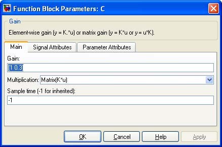
The calculations of the dumping oscillations controller X ag are taken now with the weight equal 1 while the xw pos PID controller acts with the weight 0.3. This causes, the the control algorithm mainly dumps the oscillation. The result of the experiment with the working X ag controller presents Fig. 4.43.
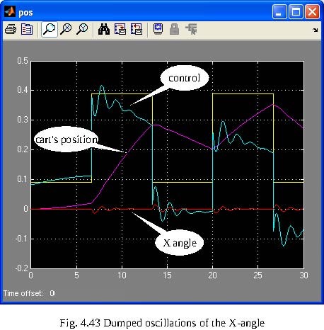
One may observe, that the oscillations are minimized by the controller, but a desired position of the cart (square wave) is tracking in a worse way then in the previous experiment.
4.4. PID simulation control of load position
In our experiment the cart is following the desired trajectory similar to Lissajous curves. We invoke the TCrane_impres model from MATLAB Command Window (see Fig. 4.44). We put the cart into motion in two directions. The desired cart positions are generated as two sinusoidal signals. There are two generators identical in amplitudes equal to 0.2 m and different in frequencies. The X motion frequency is 0.05 rad/s (Fig. 4.45) and the T angle motion frequency is 0.1 rad/s.
We perform the experiment twice, for first time without two angle controllers (X ag and Y ag). For the second time the angle controllers are included. The weights of each controller are set in the C and C1 Simulink blocks. For the first experiment we set the gains to the [0 1] values (see Fig. 4.45 and Fig. 4.46). For the second experiment we set the gains of the C and C1 block to the [0.3 1] values.
0.5 5
T ang
0 .5
0.4 5
0 .4
0.3 5
0 .3
0.2 5
0 .2
0.1 5
0 .1
X pos
0.0 5
0.05 0.1 0.15 0.2 0.25 0.3 0.35 0.4 0.45 0.5 0.55
Fig. 4.47 The desired cart positions – thin line and the cart positions – thick line (in meters)
0.2 5 0 .2 5
0 .2 0 .2
0.1 5 0 .1 5
0 .1 0 .1
X contr. vs. T contr X contr. vs. T contr
0.0 5
0 .0 5 0 0.0 5
0 .0 5 0 .1
0 .1
X ang. vs. Y ang.
X ang. vs. Y ang.
0.1 5
0 .1 5 0 .2
0 .2 0.2 5
0 .2 5
0.2 0 0.2 0.4 0.6 0.8 1 1.2 1.4 1.6 0 .2 0 0.2 0.4 0.6 0.8 1 1.2 1.4 1.6
Fig. 4.48 The controls (normalised units) and Fig. 4.49 The controls (normalised units) and the payload angles [rad] on the X Y plane; the the payload angles [rad] on the X Y plane; the angles without control angles with control
Notice that the control curve in the XT plane for the case of uncontrolled deviations of the payload is smoother than that for the controlled deviations case. The payload deviations are zoomed in Fig. 4.50 and Fig. 4.51 (please notice the scales of deviations).
3
x 10
0.0 1
6
4
0.00 5
2
0
0
2
0.00 5
4
0 .0 1
6
0.01 5
8 0 .02 0.015 0.01 0 .005 0 0.005 0.01 0.015 0.02 0.02 0.015 0.01 0.005 0 0.005 0.01 0.015
Fig. 4.50 Unstabilised deviations of Fig. 4.51 Stabilised deviations of the payload the payload in the X Y plane (in radians) in the X Y plane (in radians)
The controls in the X and T directions are shown in Fig. 4.52 and Fig. 4.53. Two cases of control: with and without stabilisation of angles are compared. The magnifications of the chosen areas are present in Fig. 4.54 and Fig. 4.55
1 .8 0 .2 5
with stbilization with stbilization
0 .2
-
1 .6
0 .1 5
-
1 .4
-
0 .1
-
0 .0 5
-
1 .2
0
1
0 .0 5
0 .1 0 .8
without stbilization
0 .1 5
0 .6
without stbilization
0 .2
0 .4
0 .2 5 0 5 10 15 20 25 30 0 5 10 15 20 25 30
Fig. 4.52 The controls (normalised units) Fig. 4.53 The controls (normalised units) in in the X direction vs. time (seconds) the T angle direction vs. time (seconds)
Notice that the controls related to the case of angles stabilisation share their actions between two tasks: tracking a desired position of the cart and stabilising the payload in its down position.
-
0 .2 2
-
0 .2
-
0 .1 8
-
0 .1 6
-
0 .1 4
-
0 .1 2
5. Prototyping your own controller in the real-time environment
In this section the process of building your own control system is described. The RTW toolbox of MathWorks and RT-CON toolbox of inteco are used. In this section we give indications how to proceed in the real-time environment.
Before starting, test your MATLAB configuration and compiler installation by building and running an example of a real-time application. TCrane toolbox includes the real-time model of PC speaker.
The model pc_speaker_xxx.mdl does not have any I/O blocks so that you can run this model regardless of the I/O boards in your computer. Running this model will test the installation by running Real-Time Workshop, and your third-party C compiler.
In the MATLAB command window, type
|
pc_speaker_vc
|
(if you are using Visual C++ compiler)
|
|
or
|
|
|
pc_speaker_watc
|
(if you are using OpenWatcom 1.3 compiler)
|
Build and run this real-time model as follows:
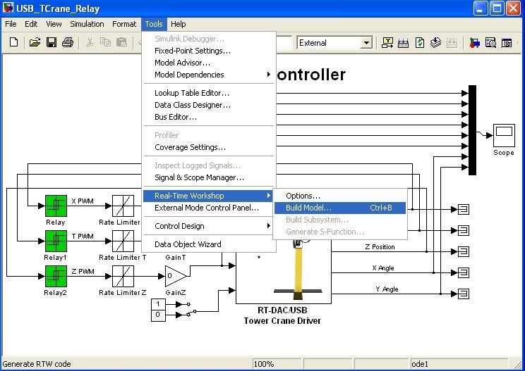
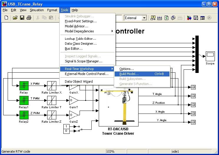
• From the Tools menu, point to Real-Time Workshop, and then click Build Model.
The MATLAB command window displays the following messages.
### Starting Real-Time Workshop build procedure for model: pc_speaker_vc
☞ ### Generating code into build directory: C:\apps\MATLAB\R2006a\work\
pc_speaker_vc_RTCON ### Invoking Target Language Compiler on pc_speaker_vc.rtw. . . . .. . . ### Created RT-CON executable: pc_speaker_vc.dll ### Successful completion of Real-Time Workshop build procedure for model:
pc_speaker_vc
• From the Simulation menu, click External, and then click Connect to target.
The MATLAB command window displays the following message. Model pc_speaker_vc loaded
• From Simulation menu, click Start real-time code.
The Dual scope window displays the output signals and you hear the speaker sound.
Only correct configuration of the MATLAB, Simulink, RTW and C compiler guaranties the proper operation of the Tower Crane system.
To build the system that operates in the real-time mode the user has to:
-
create a Simulink model of the control system which consists of the Tower Crane Driver and other blocks chosen from the Simulink library,
-
build the executable file under RTW and RT-CON (see the Tools menu in )
-
start the real-time code using menu of the model window.
5.1. Creating a model
The simplest way to create a Simulink model of the control system is to use one of the models included in the USB_TCrane_Main window as a template. For example, click on the Relay button and save it as MySystem.mdl name. The MySystem Simulink model is shown in
Now, you can modify the model. You have got absolute freedom to develop your own controller. Remember to leave the Tower Crane Device driver model.
Though it is not obligatory, we recommend you to leave the multiplexer with the scope and the control saturation blocks. You need a scope to watch how the system runs. You also need the saturation blocks to constraint the controls to match the maximal PWM signals sent to the DC motors. The saturation blocks are built in theTower Crane driver block. They limit currents to the DC motors for safety reasons. However they are not visible for the user who can be surprised that the controls saturate. Other blocks that remain in the window are not necessary for our new project.
Creating your own model on the basis of an old example ensures that all-internal options of the model are set properly. These options are required to proceed with compiling and linking in a proper way. To put the Tower Crane Device Driver into the real-time code a special make-file is required. This file is included to the Tower Crane software.
You can apply most of the blocks from the Simulink library. However, some of them cannot be used (see MathWorks references manual).
The scope block properties are important for appropriate data acquisition and watching how the system runs.
The Scope block properties are defined in the Scope property window (see Fig. 5.58). This window opens after the selection of the Scope/Properties tab. You can gather measurement data to the Matlab Workspace marking the Save data to workspace checkbox. The data is placed under Variable name. The variable format can be set asstructure or matrix. The default Sampling Decimation parameter value is set to 1. This means that each measured point is plotted and saved. Often we choose theDecimation parameter value equal to 5 or 10. This is a good choice to get enough points to describe the signal behaviour and to save the computer memory.
When the Simulink model is ready, click the Tools/External Mode Control Panel option and next click the Signal Triggering button. The window presented in Fig. 5.59 opens. Select XT Scope, set Source as manual, set Duration equal to the number of samples you intend to collect and close the window.
5.2. Code generation and the build process
Once a model of the system has been designed the code for the real-time mode can be generated, compiled, linked and downloaded into the processor.
The code is generated by the use of Target Language Compiler (TLC) (see description of the Simulink Target Language). The make-file is used to build and download object files to the target hardware automatically.
First, you have to specify the simulation parameters of your Simulink model in the Configuration parameters dialog box. The RTW page appears when you select theReal-TimeWorkshop option (Fig. 5.60). The RTW page enables to set the real-time build options and then to start the building process of the RTW.DLL executable file.
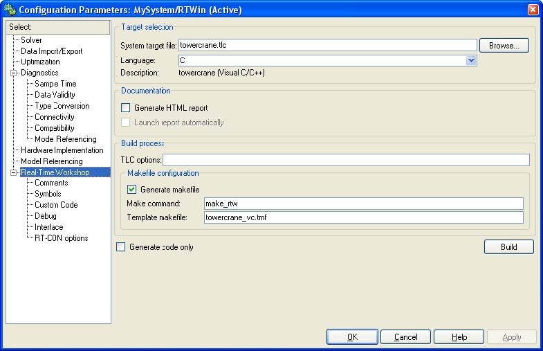
The system target file name is towercrane.tlc (for M7 R2006a/b R2007a/b, R2008a/b). It manages the code generation process. The towercrane_vc.tmf template makefile is responsible for C code generation using the open Watcom compiler.
The Solver page appears when you select the Solver option (Fig. 5.61). The Solver page enables to set the simulation parameters. Several parameters and options are available in the window. The Fixed-step size editable text box is set to 0.01 (this is the sampling period in seconds).
The Fixed-step solver is obligatory for real-time applications. If you use an arbitrary block from the discrete Simulink library or a block from the driver
☞ library remember that different sampling periods must have a common divider.
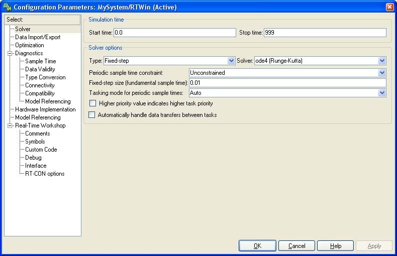
The Start time has to be set to 0. The solver has to be selected. In our example the fourth-order integration method −ode4(Runge-Kutta) is chosen.
If all parameters are set properly you can start the DLL executable building process. For this purpose press the Build push button on the RTW page (Fig. 5.60) or click Ctrl-B at keyboard being in the model window.. Successful compilation and linking processes generate the following message:
Model MyModel.rtd successfully created
### Successful completion of Real-Time Workshop build procedure for model: MyModel Otherwise, an error massage is displayed in the MATLAB command window.
Before starting the experiment set the initial position of the cart, the arm
☞ and the payload in a safe zone. The Go Home and Go To Center buttons are applied to fulfil these tasks.
6. Mathematical model of the Tower Crane
6.1. Equations
The schematic diagram related to the tower crane matheamtical model is shown in Fig.
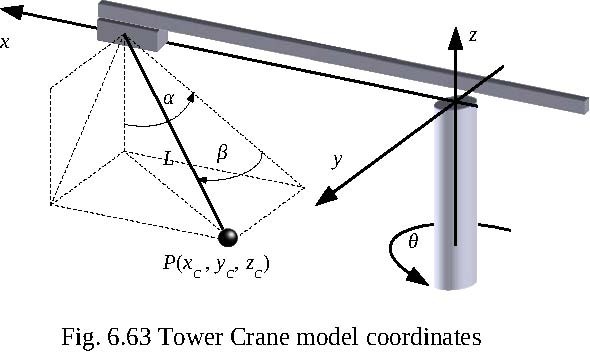
There are five measured quantities:
x
-
w denotes the distance of the cart along the arm from the center of the construction frame;
-
θ denotes the angular position of the arm
-
L denotes the length of the lift-line;
-
denotes the angle between the z axis and the projection of the lift-line onto xz plane;
-
denotes the angle between the projection of the lift-line onto the xz plane and the lift-line;
-
xc, yc, zc define coordinates of the payload.
An important element in the construction of the mathematical model is the appropriate choice of the coordinates. The center point (x=0, y=0, z=0) of the Cartesian system is in the center of the crane tower at the level equal to the suspension point of the load. The position of the payload is described by two angles, α and β , shown in Fig. 6.63. The Cartesian system rotates according to the tower movement, described by the θ angle.
It is assumed that the lift-line is permanently stretched. The position of the payload according to Fig. 6.63 is described by the formulas:
xc =xw−L cos sin (1)
y= L sin (2)
c
z=−L cos cos (3)
c
The first derivatives of the equations (1-3) and the kinetic and potential energy of the payload are calculated. Based on the Lagrange equations, Amjed A. Al-Mousa1 gives the following equations that describes the dynamics of the tower crane.
x˙1 = x5 x˙2 = x6 x˙3 = x7 x˙4 =x8
x˙5=− 1 2 g cos x2 sin x 14 x7 x8 cos x1 −L x82sin 2 x1 cos2 x2 − 2 x3 x28sin x1sin x2
2 L − 4 Lx6 x8cos x2 cos2 x1 Lx62sin 2 x1 2 sin x1 sin x2 u12 x3 cos x1 u2 − 2 L sin x2 u2
x˙6 =− 1 g sin x 2x3 x28 cos x2 −Lx82 sin x2 cos x1 cos x22 Lx5 x8 cos x1 cos x2
L cos x1
− 2 Lx5 x6sin x1 −cos x2 u1 Lsin x1cos x2 u2 x˙7 =u1 x˙8 =u2
where: x1= , x2= , x3 = xw , x4 = , x5 =˙, x6 =˙, x7 = x˙w , x8 =˙, u1 =x¨w , u2 =¨.
It is assumed that the length of the lift line L is constant.
6.2. Comparison between the mathematical model and laboratory system.
Figures 6.64 and 6.65 presents variables and directions used in the model and system.
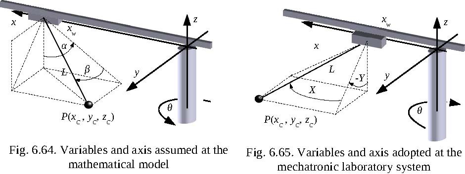
The basic differences between the model and system are as follows:
-
the control signal – it is the acceleration inside the model it is the velocity inside the system,
-
the angles of the payload – see the completely different notification in the above figures.
1 Amjed A. Al-Mousa, Control of Rotary Cranes Using Fuzzy Logic and Time-Delayed Position Feedback Control, Virginia Polytechnic Institute and State University, 27-th November 2000
• the tower rotate clockwise in the model and counterclockwise in the system.
The Tower Crane system is supplied with a Simulink block Tower Crane model that is based on the mathematical model see Fig. 6.66.
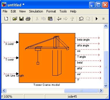
The model is equipped in two control inputs: X control and T control that correspond to the appropriate accelerations. The third input feeds a constant as the lift line length. The state variables are collected as the outputs.
Double clicking the Tower Crane model block to introduce the initial values of the ststes Fig. 6.67.
To adopt the mathematical model to the system a number of modifications of the Simulink model have been introduced (see Fig. 6.68).
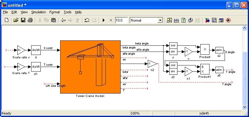
To assure a control signal compatibility (velocity – acceleration) two Simulink block Derrivative are added and two gains: Scale rate x and Scale rate T.
A conversion between the angles , and X,Y describes two formulas: X =arcsin −cos⋅sin sin
Y =arcsin −
.,
cos X
The clockwise rotation in the system and counterclockwise rotation in the model have been equalized. The gain = – 1 in the n2 block was introduced and the Scale rate T factor was multiplied by – 1 as well.
7. Description of the Tower Crane class properties
The towercrane is a MATLAB class, which gives the access to all the features of the RTDAC/USB board equipped with the logic for the Tower Crane model. The RT-DAC/USB board is an interface between the control software executed by a PC computer and the power-interface electronic of the Tower Crane model. The logic on the board contains the following blocks:
-
incremental encoder registers – five 16-bit registers to measure the position of the incremental encoders. There are five encoders measuring five state quantities: two cart positions at the cylindrical plane, the lift-line-length and two deviation angles of the payload;
-
incremental encoder resets logic. The incremental encoders are able to generate different output waves when the encoder rotates clockwise and the counter clockwise. The encoders are not able to detect the reference (“zero”) position. To determine the “zero” position the incremental encoder registers can be set to zero from the computer program or an encoder register is reset when the corresponding limit switch to the encoder is reached;
-
PWM generation block – generates three sets of signals. Each set contains the PWM output signal, the direction signal and the brake signal. The PWM prescaler determines the frequency of all the PWM waves. The PWM block logic can prevent the cart from motion outside the rail limits and the lift-line angles from lying outside the operating range. The operating ranges are detected twofold – by the limit switches and by three limit registers;
-
power interface thermal flags – when the temperature of the power interface for the DC motors is too high the thermal flags can be used to disable the operation of the corresponding overheated DC motor.
All the parameters and measured variables from the RT-DAC/USB board are accessible by appropriate methods of the towercrane class.
The object of the towercrane class is created by the command:
object_name = towercrane;
The get method is called to read a value of the property of the object:
property_value = get( object_name, ‘property_name’ );
The set method is called to set new value of the given property:
set( object_name, ‘property_name’, new_property_value );
The display method is applied to display the property values when the object_name is entered in the MATLAB command window.
This section describes all the properties of the towercrane class. The description consists of the following fields:
|
Purpose
|
Provides short description of the property
|
|
Synopsis
|
Shows the format of the method calls
|
|
Description
|
Describes what the property does and the restrictions of is
|
|
|
subjected to
|
|
Arguments
|
Describes arguments of the set method
|
|
See
|
Refers to other related properties
|
|
Examples
|
Provides examples how the property can be used
|
7.1. BaseAddress
Purpose: Read the base address of the RT-DAC/USB board.
Synopsis: BaseAddress = get( tcrane, ‘BaseAddress’ );
Description: The base address of RT-DAC/USB board is determined by OS. Each towercrane object has to know the base address of the board. When the towercrane object is created the base address is detected automatically. The detection procedure detects the base address of the first RT-DAC/USB board plugged into the USB slots.
Example: Create the towercrane object: tcrane = towercrane;
Display its properties by typing the command:
tcrane
>>Type: towercrane Object >>BaseAddress: 528 >>Bitstream ver.: x33 >>Encoder: [ 65479 7661 20032 65533 65534 ][bit] >> [ -0.0022207[m] 0.29847[m] 0.38411[m] -0.004602[rad] -0.003068[rad] ] >>Z displacement: 0.32[m] >>PWM: [ -0.062561 0.031281 -1 ] >>PWMPrescaler: 60 >>RailLimit: [ 361 381 815 ]*64[bit] <--> [23104 24384 52160 ][bit] >> [ 0.90013 0.95 1.0002 ][m] >>RailLimitFlag: [ 1 1 1 ] >>RailLimitSwitch: [ 0 1 1 ] >>ResetSwitchFlag: [ 0 0 0 ] >>Therm: [ 1 1 1 ]>>ThermFlag: [ 1 1 1 ] >>Time: 1.041 [sec]
Read the base address:
BA = get( tcrane, ‘BaseAddress’ );
7.2. BitstreamVersion
Purpose: Read the version of the logic design for the RT-DAC/USB board.
Synopsis: Version = get( tcrane, ‘BitstreamVersion’ );
Description: This property determines the version of the logic design of the RTDAC/USB board. The Tower Crane models may vary and the detection of the logic design version makes it possible to check if the logic design is compatible with the physical model.
7.3. Encoder
Purpose: Read the incremental encoder registers.
Synopsis: enc = get( tcrane, ‘Encoder’ );
Description: The property returns five digits. The first two measure the position of the cart – linear and angle. The third digit is used to measure the length of the lift-line and the last two measure the angles of the lift-line. The returned values can vary from 0 to 65535 (16-bit counters). When a register is reset the value is set to zero. When a rail limit flag is set it disables the movement outside the defined working range (rail limit). When a reset switch flag is set the encoder register is reset automatically when the appropriate switch is pressed.
The incremental encoders generate 4096 or 2048 pulses per rotation. The values of the Encoder property should be converted into physical units.
See: ResetEncoder, RailLimit, RailLimitFlag, ResetSwitchFlag
7.4. PWM
Purpose: Set the parameters of the PWM waves.
Synopsis: PWM = get( tcrane, ‘PWM’ ); set( tcrane, ‘PWM’, NewPWM );
Description: The property determines the duty cycle and direction of the PWM waves for three DC motors. The first two DC motors control the position of the cart and the last motor controls the length of the lift-line. The PWM and NewPWM variables are 1x3 vectors. Each element of these vectors determines the parameters of the PWM wave for one DC motor. The values of the elements of these vectors can vary from –1.0 to 1.0. The value –1.0 means the maximum control in one direction, the value 0.0 means zero control and the value 1.0 means the maximum control in the opposite direction.
The PWM wave is not generated if:
-
a rail limit flag is set and the cart or lift-line are going to operate outside the working range,
-
a therm flag is set and the power amplifier is overheated.
See: RailLimit, RailLimitFlag, Therm, ThermFlag
Example: set( tcrane, ‘PWM’, [ -0.3 0.0 1.0 ] );
7.5. PWMPrescaler
Purpose: Determine the frequency of the PWM waves.
Synopsis: Prescaler = get( tcrane, ‘PWMPrescaler’ ); set( tcrane, ‘PWMPrescaler’, NewPrescaler );
Description: The prescaler value can vary from 0 to 63. The 0 value generates the maximum PWM frequency. The value 63 generates the minimum frequency.
See: PWM
7.6. ResetEncoder
Purpose: Reset the encoder counters.
Synopsis: set( tcrane, ‘ResetEncoder’, ResetFlags );
Description: The property is used to reset the encoder registers. The ResetFlags is a 1x5 vector. Each element of this vector is responsible for one encoder register. If the element is equal to 1 the appropriate register is set to zero. If the element is equal to 0 the appropriate register remains unchanged.
See: Encoder
Example: To reset the first and fourth encoder registers execute the command: set( tcrane, ‘ResetEncoder’, [ 1 0 0 1 0 ] );
7.7. RailLimit
Purpose: Control the operating range of the tower crane system.
Synopsis: Limit = get( tcrane, ‘RailLimit’ ); set( tr3, ‘RailLimit’, NewLimit );
Description: The Limit and NewLimit variables are 1x3 vectors. The elements of these vectors define the operating range of the cart and the maximum length of the lift-line. If a flag defined by the RailLimitFlag property is set the corresponding to it PWM wave stops when the corresponding to it encoder register exceeds the limit.
See: RailLimitFlag
7.8. RailLimitFlag
Purpose: Set range of limit flags.
Synopsis: LimitFlag = get( tcrane, ‘RailLimitFlag’ ); set( tr3, ‘RailLimitFlag’, NewLimitFlag );
Description: The RailLimitFlags is a 1x3 vector. The first two elements control the operating range of the cart (a length of the rail and an angle position of the tower). The last element controls the maximum length of the lift-line. If the flag is set to 1 and the encoder register exceeds the range the DC motorcorresponding to it stops. If the flag is set to 0 the motion continues in spite of the range limit exceeded in the encoder register.
See: RailLimit, RailLimitSwitch
7.9. RailLimitSwitch
Purpose: Read the state of limit switches. Synopsis: LimitSwitch = get( tcrane, ‘RailLimitSwitch’ ); Description: Reads the state of three limit switches. Returns a 1x3 vector. If an element of
this vector is equal to 0 it means that the switch has been pressed.
See: RailLimit, RailLimitFlag
7.10. ResetSwitchFlag
Purpose: Control the auto-reset of the encoder registers.
Synopsis: ResetSwitchFlag = get( tcrane, ‘ResetSwitchtFlag’ ); set( tcrane, ‘ResetSwitchFlag’, ResetSwitchFlag );
Description: The ResetSwitchFlag and NewResetSwitchFlag are 1x3 vectors. If an element of these vectors is equal to 1 the corresponding to it encoder register is automatically reset in the case when the corresponding to it limit switch is pressed.
See: ResetEncoder, RailLimitSwitch
7.11. Therm
Purpose: Read thermal flags of the power amplifiers. Synopsis: Therm = get( tcrane, ‘Therm’ ); Description: Returns three thermal flags of three power amplifiers. When the temperature
of a power amplifier is too high the appropriate flag is set to x.
See: ThermFlag
7.12. ThermFlag
Purpose: Control an automatic power down of the power amplifiers.
Synopsis: ThermFlag = get( tcrane, ‘ThermFlag’ ); set( tcrane, ‘ThermFlag’, NewThermFlag );
Description: The ThermFlag and NewThermFlag are 1x3 vectors. If an element of these vectors is equal to 1 the DC motor corresponding to it is not excited by the PWM wave when it is overheated.
See: Therm
7.13. Time
Purpose: Return time information.
Synopsis: T = get( tcrane, ‘Time’ );
Description: The towercrane object contains the time counter. When a towercrane object is created the time counter is set to zero. Each reference to the Timeproperty updates its value. The value is equal to the number of milliseconds past since the object was created.
7.14. Quick reference table
|
Property Name
|
Description
|
|
BitstreamVersion
|
Read the version of the logic design for the RT-DAC/USB board
|
|
Encoder
|
Read the incremental encoder registers
|
|
PWM
|
Set the parameters of the PWM waves
|
|
PWMPrescaler
|
Determine the frequency of the PWM waves
|
|
ResetEncoder
|
Reset the encoder counters
|
|
RailLimit
|
Control the operating range of the Tower Crane system
|
|
RailLimitFlag
|
Set the range limit flags
|
|
RailLimitSwitch
|
Read the state of the limit switches
|
|
ResetSwitchFlag
|
Control the auto-reset of the encoder registers
|
|
Therm
|
Read the thermal flags of the power amplifiers
|
|
ThermFlag
|
Control the automatic power down of the power amplifiers
|
|
Time
|
Return time information
|
8. How to fill in the compilation settings page
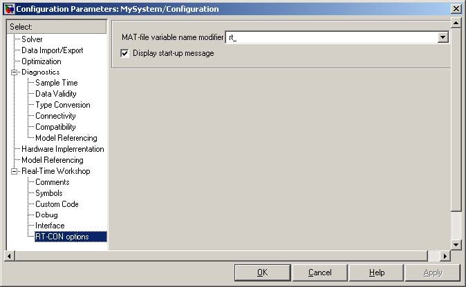
In Fig. 8.69 and Błąd: Nie znaleziono źródła odwołania the Configuration Parameters pages for different MATLAB versions are shown.

Notice that system target file towercrane.tlc (rtcon.tlc) is chosen. Also note that template makefile, responsible for compilation and linking process, istowercrane_vc.tmf (rtcon_vc_usb.tmf). It means the MS VC++ compiler is used in this case.
Interface page, responsible for connection with external target system, is shown in Fig.
8.70. To fulfil it properly a user must select External mode in Interface edit window. After that the user have to set RT-CON tcpip in the Transport layer edit window.
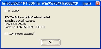
If this checkbox is marked the message on loading real-time code is displayed (Fig. 8.72) after connecting to target in the model window.
 收藏灵猫网
收藏灵猫网