The laboratory Anti-lock Braking System controlled from PC
Getting Started

Printed by inteco Ltd
phone./fax: (48) 12 430-49-61, e-mail: Inteco@kki.krakow.pl
CONTENTS
1. INTRODUCTION AND GENERAL DESCRIPTION ............................................................................ 3
1.1. Product overview................................................................................................................................... 4
1.2. Requirements......................................................................................................................................... 4
2. INSTALLATION OF THE SOFTWARE................................................................................................. 5
3. STARTING, TESTING AND STOPPING PROCEDURES ................................................................... 5
3.1. Starting procedure.................................................................................................................................. 5
3.2. Testing ................................................................................................................................................... 5
3.3. Stopping procedure................................................................................................................................ 7
4. MAIN CONTROL WINDOW ................................................................................................................... 7
4.1. Tools...................................................................................................................................................... 7
4.2. RTWT Device Driver ............................................................................................................................ 9
4.3. Simulation model................................................................................................................................. 11
4.4. Demo Controller .................................................................................................................................. 12
5. PROTOTYPING YOUR OWN CONTROLLER IN THE RTWT ENVIRONMENT....................... 18
5.1. Creating a model.................................................................................................................................. 19
5.2. Code generation and the build process ................................................................................................ 20
6. MATHEMATICAL MODEL................................................................................................................... 23
6.1. Equations of motion............................................................................................................................. 25
6.2. Identification........................................................................................................................................ 27
6.2.1. Geometrical issues.................................................................................................. 27
6.2.2. Deriving of torque Mg .......................................................................................... 27
6.2.3. Derivations of moments of inertia.......................................................................... 28
6.2.4. Derivingthe friction coefficients in the bearings...................................................29
6.2.5. Identification of the friction coefficient and the braking torque ............................ 30
7. SIMULATION OF BRAKING ................................................................................................................ 33
1. Introduction and general description
The anti-lock braking system (ABS) in cars were implemented in the late 70’s. The main objective of the control system is to prevent of wheel-lock while braking. Usually we are interested in the tire slip on each of the four wheels in the car. Only longitudinal motion is considered. Nevertheless differences between the front and the back wheels and between the right and the left wheels, we consider only a simplified model of the quarter car.
ABS are designed to optimize braking effectiveness while maintaining car controllability. The performance of ABS can be demonstrated in our lab-set by simulation for various road condition (wet asphalt) and transition between such conditions (e.g., when emergency braking occurs and the road switches from dry to wet or vice versa).
ABS is driven by the powerful, flat DC motor. There are three identical encoders measuring the rotational angles of two wheels and the deviation angle of the balance lever of the car wheel. The encoders measure movements with a high resolution equal to 4096 pulses per rotation.
The power interface amplifies the control signals which are transmitted from the PC to the DC motor. It also converts the encoders pulse signals to the digital 16-bit form to be read by the PC. The PC equipped with the RT-DAC4/PCI-D multipurpose digital I/O board communicates with the power interface. The whole logic necessary to activate and read the encoder signals and to generate the appropriate sequence of pulses of PWM to control the DC motor is configured in the Xilinx® chip of the RT-DAC4/PCI-D board. All functions of the board are accessed from the ABS Toolbox which operates directly in the MATLAB®/ Simulink® and the RTWT toolbox environment
At the beginning of an experiment the wheel animating the relative car-road motion is accelerated to a given threshold velocity. The wheel accelerates following the rotational motion of the "car-road" wheel. Next, the DC drive is switched off to enable free motion of both wheels. In fact, there are two threshold velocities during the acceleration of the wheels. The first threshold velocity is introduced to the power interface to prevent a large starting current value. At the beginning the DC motor is supplied in series by a starting resistor from the power interface. If the first threshold velocity of the motor is reached then the starting resistor is switched off and the DC motor is supplied directly from the power interface. If the second threshold velocity (defined in the program and of course with the higher value than the first one) is reached then the power interface is switched off and the braking phase begins.
To understand the braking process one has to know relations between the vehicle tire and road during braking. The objective of ABS is to control wheel slip to maximize the coefficient of friction between the tire and road for any given road surface while the car is controllable.
If this wheel becomes motionless it means that it remains in slip motion (the car velocity is not equal to zero) or is absolutely stopped (the car velocity is equal to zero). In the first case the ABS algorithm has to unlocked the wheel to stop its slipping. The wheel starts to rotate and after a short time period it is stopped again. This process is repeated as long as the car velocity achieves zero value (the wheel animating the road motion related to car is stopped). If the braking time period is too long the wheel remains locked in slip motion and the car starts an uncontrollable motion. If this period is too short the wheel remains to long in the rolling stage and the brake distance is also enlarged.
1.1. Product overview
ABS is delivered in mounted form. The mounting frame makes a support of the system. It is ready to operate after installation of its software.
KEY FEATURES
-
Double-wheel laboratory model of ABS equipped with powerful, flat dc motor.
-
Three high-resolution measuring encoders.
-
Full integration with MATLAB®/ Simulink®. Operation in real-time in MS Windows® 98/NT/2000/XP.
-
Complete model of the car-road relations.
-
Library of pre-programmed braking control algorithms familiarize the user with ABS technique in a fast way.
-
Rapid prototyping of real-time control algorithms. No C-code programming.
-
Ideal illustration of nonlinear control algorithms.
KEY BENEFITS
-
Enables to provide laboratory tests of the antilock braking system in the car velocity range from 0 to 50 km/h.
-
Accelerates implementation of new slip control algorithms.
-
Demonstrates slip control under different road conditions.
SETUP COMPONENTS
hardware
-
mechanical unit (frame, double wheel, DC flat motor),
-
interface and Power Interface Unit
-
I/O RT-DAC/PCI-D board (the PWM control logic is stored in a XILINX chip)
software
• ABS Control/Simulation Toolbox operating in MATLAB®/Simulink® environment
manuals
-
Installation Manual
-
Getting Started Manual
1.2. Requirements
-
INTEL or AMD based PC,
-
Video card resolution 1024 x 768 pixels
-
MATLAB® 6.x /Simulink® 4.x,
-
Real Time Workshop and Real Time Windows Target toolboxes
-
Compiler: MS Visual C ++
 The ABS toolbox supports Matlab 6.x with the MS Visual C++ compiler.
2. Installation of the software
Put the installation disc into your computer and follow the installation procedure step by step.
3. Starting, testing and stopping procedures
3.1. Starting procedure
Combine the acquisition board, Power Interface and ABS together. In the WINDOWS environment invoke MATLAB by double clicking on the MATLAB icon. The MATLAB command window opens. Then simply type:
abs_main
MATLAB brings up the ABS Main Control Window (see Fig. 3.1). Pushbuttons indicate an action that executes callback routines when the user selects a menu item.
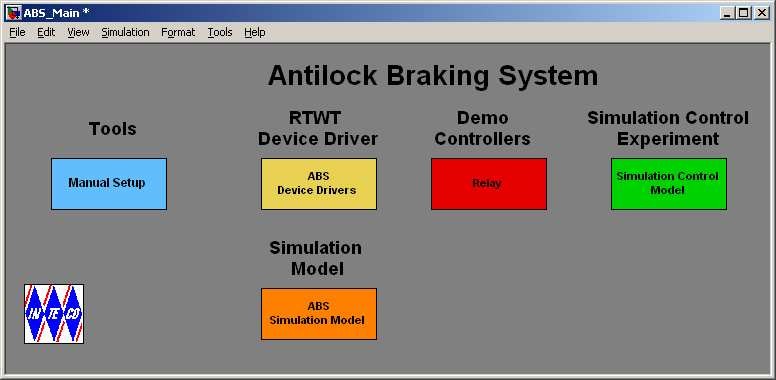
The Main Control Window contains testing tools, drivers, models and demo applications. You can see a number of pushbuttons ready to use.
3.2. Testing
Double click the Manual Setup button to check connections of all components of the system. The screen given in Fig. 3.2 opens. In the left upper corner box there are two text information fields: Base Address andBitstream Version. Non zero data in these fields indicates that the RT-DAC4/PCI-D board has been correctly detected by the system. We can notice that the measurement data in this window are equal to zero. Now the following test is recommended. Change slightly the position of the Acceleration slider. The DC motor turns around. Click the Update button and Stop button. You can notice that new measurement data have appeared (see Fig. 3.3). If the new data are not visible it means that the system is assembled in a wrong way. In such a case please come back to the Installation Manual and check the connections again.
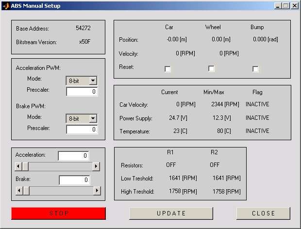

 Remember Car in Fig. 3.2 and Fig. 3.3 denotes the lower wheel of the system. Wheel denotes the upper wheel.
3.3. Stopping procedure
The system is equipped with the hardware stop pushbutton. It cuts off the control transfer signal to the system drive. The pushbutton does not terminate the real-time process running in the background. Therefore to stop the task you have to use Simulation/Stop from the pull-down menus in the model window.
4. Main Control Window
The user has a rapid access to all basic functions of ABS from the Main Control Window. It includes tools, drivers, models and application examples.
The Main Control Window shown in Fig. 3.1 contains:
-
Tools
-
RTWT Device Driver
-
Simulation model
-
Demo Controllers
-
Simulation Control Experiment
4.1. Tools
One can change the ABS MATLAB structure using the Manual Setup – GUI interface. Double click the Manual Setup button and the screen given in Fig. 4.1 opens.
 Remember Car in Fig. 4.1 denotes the lower wheel of the system. Wheel denotes the upper wheel.

There are numerical data in the window read from the XILINX chip placed on the RTDAC4/PCI-D board. These data reflects the MATLAB structure, which includes measurements and constants assumed in the system.
In the first frame there is the basic information:
-
Base Address – the autodetected base address of the RT-DAC/PCI-D board,
-
Bitstream ver. − the version of the logic design for the RT-DAC/PCI-D board.
The second frame contains the information corresponding to the acceleration and brake PWM settings:
Acceleration PWM
-
Mode – 12-bits or 8-bits acceleration PWM mode.
-
Prescaler – the frequency of the acceleration PWM (pulse width modulation) waves. Brake PWM
-
Mode – 12-bits or 8-bits brake PWM mode.
• Prescaler – the frequency of the brake PWM (pulse width modulation) waves. The next frame includes the control sliders for the acceleration and brake processes.
• They are used to control manually the acceleration and the brake of the wheel. Note, that after opening this window all controls are set to zero. Change the positions of the sliders and observe acceleration and brake processes in the system. To stop the experiment click the STOP button. The system will stop and all sliders return to the zero positions.
The next frame contains the encoder measurements:
-
Positions of the both wheels expressed in meters and bumps of the balance lever expressed in radians.
-
Velocities of the both wheels expressed in RPM. They are updated and refreshed when the UPDATE button is pushed.
-
Marking the reset checkbox result in resetting of the encoder corresponding to that mark.
The consecutive frame shows the following measurements:
-
Current Car Velocity and its maximal admissible value. If the car velocity reaches maximal value the accelerating is stopped and braking process starts.
-
Current voltage of the Power Supply and its minimal acceptable value. If the voltage is under the minimum the power interface is turned off.
-
Current Temperature value of the power supply and its upper limit. If temperature reaches the upper limit the power supply is turned off. It can be turn on again if the temperature falls down under the upper limit value.
-
The Flag column shows if the suitable event occurs. The INACTIVE caption means that the corresponding limits have not been reached. The red ACTIVE caption indicates that the limit has been reached.
The next frame indicates if the acceleration resistors of the power interface are switched on.
• When the big DC motor driving the road wheel starts a starting current must be constrained. It is realized by switching on/off the R1 and R2 starting resistors involved into the power interface. They are turned on or off when the current car velocity reaches the Low Treshold and High Treshold. Too large starting current might result in a damage of the power interface.
The UPDATE button has to be clicked to read the current values of the all measurements accessible from the Manual Setup window.
4.2. RTWT Device Driver
The driver is a software go-between for the real ABS system MATLAB environment and the RT-DAC/PCI-D acquisition board. This driver serves to the control and measurement signals. Click the ABS Device Driver button and the driver window opens (Fig. 4.2)
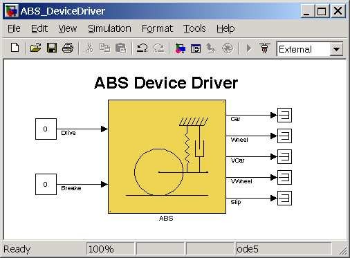
The driver has two inputs: PWM input -Drive (DC motor control) and Brake (brake control). There are 5 outputs of the driver: Car position (Car) , Wheel position (Wheel), Car Velocity (Vcar), Wheel Velocity (VWheel) and Slip. When one wants to build ones own application one can copy this driver to a new model.
 Do not do changes inside the original driver. They can be done only inside its copy!!!
4.3. Simulation model
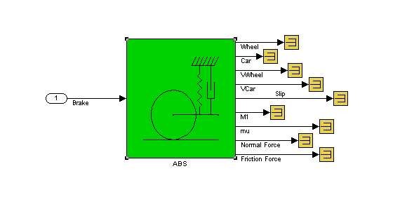
The simulation model of the ABS is accessible from the ABS Simulation Model button. Its external (see Fig. 4.3) is very similar as the model given in the ABS Device Driver. Notice, that model has only one input denotedBrake. If we use the simulation model it is not necessary to accelerate the system. We set non zero initial velocities and begin the braking procedure. If we compare the simulation model to the ABS Device Driver we notice that four outputs are added to the model. These outputs are described in the section 6. The simulation model is used for many purposes: identification, design of controllers, etc. The interior of the simulation model is given in Fig. 4.4. There are two integrators introduced to obtain angular positions from angular velocities. Two gain blocks are used to calculate the appropriate units.
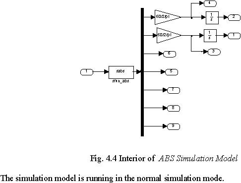
 Set solver options to: Fixed step and Fixed-step size equal to 0.01. The Runge-Kutta solver is recommended.
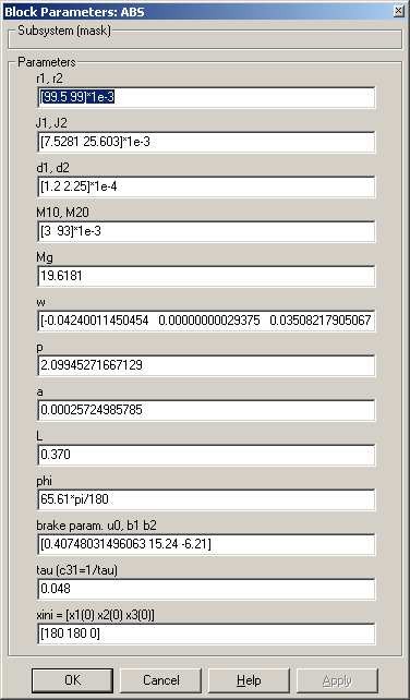
In the mask presented in Fig. 4.5 you can set all coefficients of the model and introduce initial conditions for the model state variables. See section 6 for details.
4.4. Demo Controller
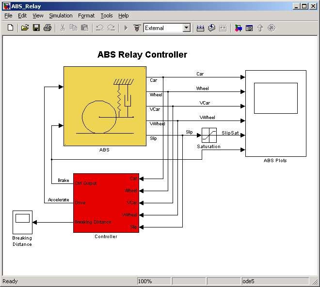
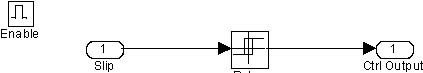
In this column examples of control systems are given. These demos can be used to familiarise the user with the ABS operation and allow to create the user-defined control systems. The examples must be rebuilt before using. Due to similarity of the examples we focus our attention on one of them. After clicking on the Relay button the model shown in Fig. 4.6 appears. Notice that this model looks like a typical Simulink model. The device driver is applied in the same way as other blocks from the Simulink library. The only difference is that the model is used by Real Time Windows Target (RTWT) to create the executable library, which runs in the real-time mode.
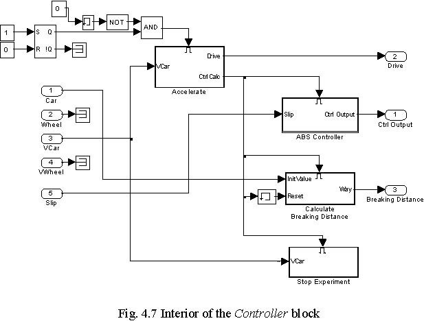
Click Controller block and next type Ctrl U . The interior of the Controller block shown in Fig. 4.7 appears. Pay attention that some blocks in Fig. 4.7 are the Enable type. These are: Acceleration block, ABS Controller block, Calculate braking distance and Stop experiment block. How the experiment is performed? At the beginning the Acceleration block is enabled. The DC motor is controlled and the wheel is accelerated until the angular velocity of the wheel reaches the velocity limit. The proper logic is placed in the Acceleration block. If the Acceleration block halts then it enables three next blocks: the ABS Controller block, Calculate braking distance and Stop experiment block. The names of the blocks correspond to the functions realized by them. The braking action runs until the car is stopped. The relay controller is applied. The interior of the ABS Controller block is given in Fig. 4.8.
Stop Experiment
We are ready now to return to the model window (see Fig. 4.6) and click the Controller block. The mask shown in Fig. 4.9 opens.
Relay

Fig. 4.9 Parameters of the relay controller
Velocity Treshold [RPM] equal to 2300 means: if velocity reaches 2300 RPM the wheel acceleration is stopped and the braking of the wheel starts. Switch point [)N OFF] equal to [0.1 0.1] means: if the slip is greater than 0.1 the relay turns on the brake, and if the slip is less than 0.1 the relay turns off the brake. Control When [ON OFF] equal to [0 1] means the control is equal to 0 when Switch Point is ON and the control is equal to 1 when Switch Point is OFF.
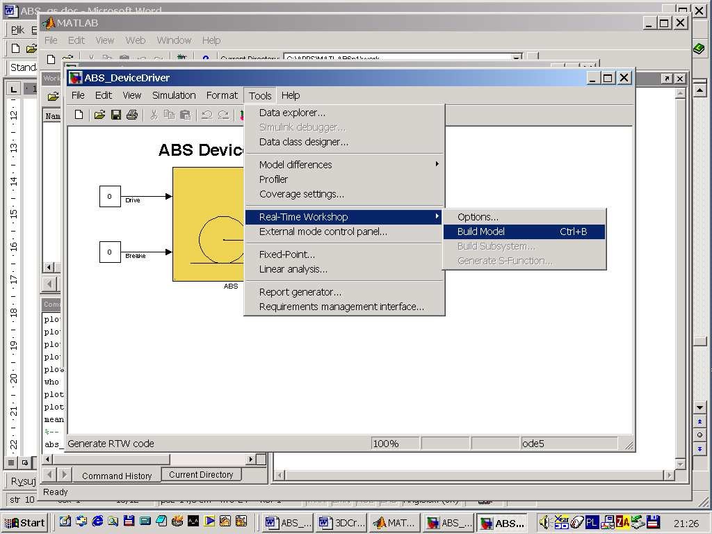
Then, choose the Tools pull-down menu in the Simulink model window. The pop-up menu provide a choice between predefined items. Choose the RTW Build item. A successful compilation and linking processes are finished with the following message:
Model ABS_Relay.rtd successfully created
### Successful completion of Real-Time Workshop build procedure for model:
ABS_Relay
If an error occurs then the message corresponding to this error is displayed in the MATLAB command window.
Now, we return to the model window and click the Simulation/Connect to Target option. Next, click the Simulation/Start real-time code item.
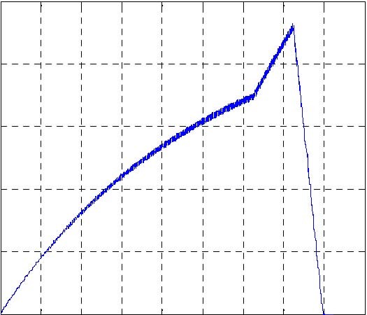
The system starts and the wheel accelerates. When the car velocity reaches upper limit (1700 rpm) the acceleration stops and the braking begins. This is visible in the plots in the scope. The experiment stops after 20 seconds.
Results displayed in the scope are stored as the structure with time in the variable ABSHistory (it has been set in the option of the scope ABS plots). In order to plot the results we can write in Matlab Command Window:
t=ABSHistory.time;
vcar=ABSHistory.signals(3).values;
slip=ABSHistory.signals(5).values;
plot(t,vcar);grid;title(‘Car velocity’);xlabel(‘time [sec]’);
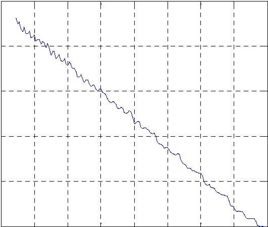
plot(t,slip);grid;title(‘Slip’);xlabel(‘time [sec]’);
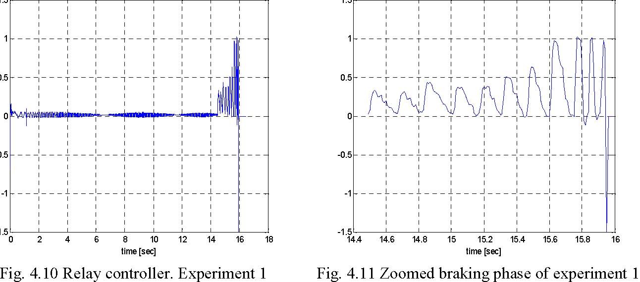
All experimental results related to acceleration and braking are shown in Fig. 4.10.
a = 1450; b = 1600;
plot(t(a:b),vcar(a:b));grid;title(‘Car velocity -braking time’);xlabel(‘time [sec]’);
plot(t(a:b),slip(a:b));grid;title(‘Slip -braking time’);xlabel(‘time [sec]’);
The braking phase of the experiment 1 in the zoomed form is shown in Fig. 4.11.
Car velocity Car velocity -braking time 2500
 2500
2500
2000
2000
1500
1500
1000
1000
500 500
0
0 0 2 4 6 8 10 12 14 16 18 14.4 14.6 14.8 15 15.2 15.4 15.6 15.8 16
time [sec] time [sec]
Slip Slip -braking time
1.5
 1.5
1.5
1 1
0.5
0.5
0 0
-0.5
-0.5
-1 -1
-1.5
-1.5 0 2 4 6 8 10 12 14 16 18 14.4 14.6 14.8 15 15.2 15.4 15.6 15.8 16
time [sec] time [sec]
The braking distance, read out from the Breaking Distance scope is equal to 17.7 m. We can notice the time moments at the car velocity plot in which the starting resistors are turned off. We can also notice that negative slip values may appear in the plot. If small velocities are observed the numerical data are not accurate. Note that the slip often reaches zero (see Fig. 4.11). It means that in these moments the braking is off and the brake is released. In this case the braking distance is long and it shows that the applied control algorithm does not fit well to the braking task.
In this demo one can try to adjust the parameters of the control algorithm. Click Controller block and set Switch point to [0.7 0.7] (see Fig. 4.9). Next return to the model window and click theSimulation/Connect to Target option. Next, click the Simulation/Start real-time code item.
Acceleration and braking experimental results are shown in Fig. 4.12. The braking phase of the experiment in the zoomed form is given in Fig. 4.12.
Car velocity
2500
2000
1500
1000
500
0
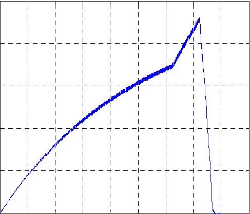
0 2 4 6 8 10 12 14 16 18 time [sec]
Slip
1.5
1
0.5
0
-0.5
-1
-1.5
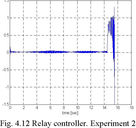
0 2 4 6 8 10 12 14 16 18 time [sec]
Car velocity -braking time
2500
2000
1500
1000
500
|
14.4 0
|
14.6
|
14.8
|
15
|
15.2 time [sec]
|
15.4
|
15.6
|
15.8
|
16
|
|
1.5
|
|
|
Slip -braking time
|
|
|
|
1
0.5
0
-0.5
-1
-1.5
14.4 14.6 14.8 15 15.2 15.4 15.6 15.8 time [sec]
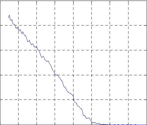

Comparing the experimental results of Experiment 1 to Experiment 2 we can notice the similar car velocity plots and very different slip plots. The braking distance read from the Breaking Distance scope is equal to 12 m. This result is better than that obtained in the previous experiment. Note that the slip is equal to zero or negative only at the end of the braking zone when the car velocity is very small.
5. Prototyping your own controller in the RTWT environment
In this section the process of building of your own control system is described. The Real Time Windows Target (RTWT) toolbox is used. An example how to use the ABS software is shown in section 4.4. In this section we give indications how to proceed in the RTWT environment. We assume a user is familiarised with Matlab, Simulink and RTW/RTWT toolboxes.
 Before a start, test your MATLAB configuration and compiler installation by building and running an example of a real-time application. Real-time
Windows Target includes the model rtvdp.mdl. Running this model will test the installation by running Real-Time Workshop, your third-party C compiler, Real-Time Windows Target, and the Real-Time Windows Target kernel. In the MATLAB Command Window, type
rtvdp
Next, build and run the real-time model. For details refer to the Real-Time Windows Target help, section Installation and Configuration.
To build the system that operates in the real-time mode the user has to:
-
create a Simulink model of the control system which consists of the ABS system Device Driver and other blocks chosen from the Simulink library,
-
built the executable file under RTWT (see the pop-up menu in Fig. 5.1)
-
start the real-time code to run from the Simulation/Start real-time code pull-down menu.
5.1. Creating a model
The simplest way to create a Simulink model of the control system is to use one of the models included in the Main Control Window as a template. For example, click on the Relay button and save it asMySystem.mdl name. The MySystem Simulink model is shown in Fig.
5.2.
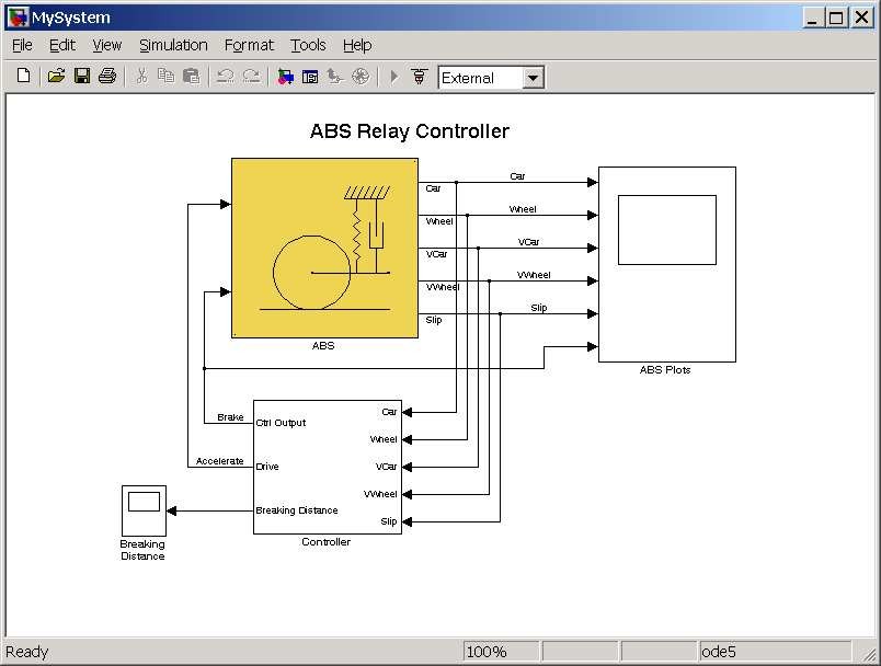
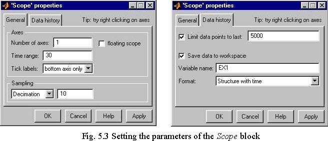
Now, you can modify the model. You have absolute freedom to develop your own controller. Remember to leave the ABS system driver model in the window. Though it is not obligatory, we recommend to you to live the scope block. You need a scope to watch how the system runs. Other blocks remaining in the window are not necessary for our new project. Creating your own model on the basis of an old example ensures that all-internal options of the model are set properly. These options are required to proceed with compiling and linking in a proper way. To put the ABS system Device Driver into the real-time code a special make-file is required. This file is included into the ABS system software. You can apply almost all of the blocks from the Simulink library. However, some of them cannot be used (see MathWorks references manual). The scope block properties are important for an appropriate data acquisition and watching how the system runs. The Scope block properties are defined in the Scope property window (see Fig. 5.3). This window opens after the selection of theScope/Properties tab. You can gather measurement data to the Matlab Workspace marking the Save data to workspace checkbox. The data is placed under Variable name. The variable format can be set as structureor matrix. The default Sampling Decimation parameter value is set to 1. This means that each measured point is plotted and saved. Often we choose the Decimation parameter value equal to 5 or 10. This is a good choice to get enough points to describe the signal behaviour and simultaneously to save the computer memory.
5.2. Code generation and the build process
Once a model of the system has been designed the code for real-time mode can be generated, compiled, linked and downloaded into the processor. The code is generated by the use of Target Language Compiler (TLC) (see description of the Simulink Target Language). The make-file is used to build and download object files to the target hardware automatically. First, you have to specify the simulation parameters of your Simulink model in the Simulation parameters dialog box. The RTW page appears when you select the RTW tab (Fig. 5.4). The RTW page allows you to set the real-time build options and then to start the building process of the RTW.DLLexecutable file.
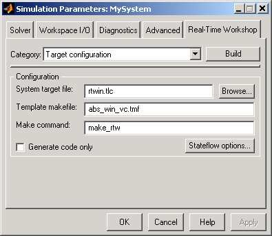
The system target file name is rtwin.tlc. It manages the code generation process. Notice that the abs_win_vc.tmf template make-file is also included to the software. It is ready to be used by the Microsoft Visual C++ 6.0 compiler.
There is additional option Generate code only which have to be properly marked as shown in Fig. 5.4. If marked, a code is generated but compilation is not performed.
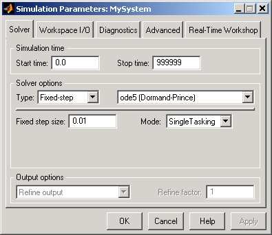
The Solver page appears when you select the Solver tab (Fig. 5.5). The Solver page allows you to set the simulation parameters. Several parameters and options are available in the window. The Fixed-step sizeeditable text box is set to 0.01 (this is the sampling period in seconds).
 The Fixed-step solver is obligatory for real-time applications. If you use an arbitrary block from the discrete Simulink library remember that different
sampling periods must have a common divider.
The Start time has to be set to 0. The solver has to be selected. In our example the fifth-order integration method − ode5 is chosen.
If all parameters are set properly you can start the DLL executable building process. For this purpose press the Build push button on the RTW page (Fig. 5.4). Successful compilation and linking processes generate the following message:
Model MyModel.rtd successfully created ### Successful completion of Real-Time Workshop build procedure for model: MyModel
Otherwise, an error massage is displayed in the MATLAB command window.
6. Mathematical model
Consider the system depicted in Fig. 6.1.
y
|
M 1
|
J 1
|
ω 1
|
|
|
r 1
|
|
F nµ
|
|
|
F nµ
|
|
|
r
|
|
|
|
|
2
|
|
|
|
|
|
ω 2
|
|
x
|
|
|
|
J
|
|
|
|
|
|
2
|
|
|
Fig. 6.1 Schematic diagram of ABS
There are two rolling wheels. The lower car-road wheel animating relative road motion and the upper car wheel permanently remaining in a rolling contact with the lower wheel. The wheel mounted to the balance lever is equipped in a tyre. The car-road wheel has a smooth surface which can be covered by a given material to animate a surface of the road.
There are three angles measured by three encoders. The accuracies of measurements are 2π/2048 = 0.175°. Τhe two first are rotational angles of the wheels. The third measurement is the angle between subsequent balance lever angular positions. This one might be used in more complex models of ABS. The wheel angular velocities are not measured. They have to be observed. The simplest Euler formula is used. The sample time is defined as 0.5 ms.
The upper wheel is equipped in the disk brake system connected via hydraulic coupling to the brake lever which by the tight side and tightening pulley is driven by the small DC motor. The lower wheel is coupled to the big flat DC motor which is power supplied to accelerate the wheel. During the braking phase the power supply is switched off. Both big and small DC motors are controlled by PWM (pulse-width modulation) signals of the 3.5 kHz frequency. The varying pulse-width is the control variable.
We define the car velocity to be equivalent to the angular velocity of the lower wheel multiplied by the radius of this wheel. We define the angular velocity of the wheel to be equivalent to the angular velocity of the upper wheel.
The state variables and parameters of the model are given in Table1.
Table 1. Parameters of the model
|
Name
|
Description
|
Units
|
|
x1
|
angular velocity of the upper wheel
|
rad/s
|
|
x2
|
angular velocity of the lower wheel
|
rad/s
|
|
M1
|
braking torque
|
Nm
|
|
r1
|
radius of the upper wheel
|
m
|
|
r2
|
radius of the lower wheel
|
m
|
|
J1
|
moment of inertia of the upper wheel
|
kgm2
|
|
J2
|
moment of inertia of the lower wheel
|
kgm2
|
|
d1
|
viscous friction coefficient of the upper wheel
|
kgm2/s
|
|
d2
|
viscous friction coefficient of the lower wheel
|
kgm2/s
|
|
nF
|
total force generated by the upper wheel and pressing on the lower wheel
|
N
|
|
µ(λ)
|
friction coefficient between wheels
|
|
|
λ
|
slip – the relative difference of the wheel velocities
|
|
|
nF
|
normal force – the upper wheel acting on the lower wheel
|
N
|
|
µ(λ)
|
friction coefficient between the wheels
|
|
|
λ
|
slip – the relative difference of the wheels velocities
|
|
|
M10
|
static friction of the upper wheel
|
Nm
|
|
M 20
|
static friction of the lower wheel
|
Nm
|
|
gM
|
gravitational and shock absorber torques acting on the balance lever
|
Nm
|
|
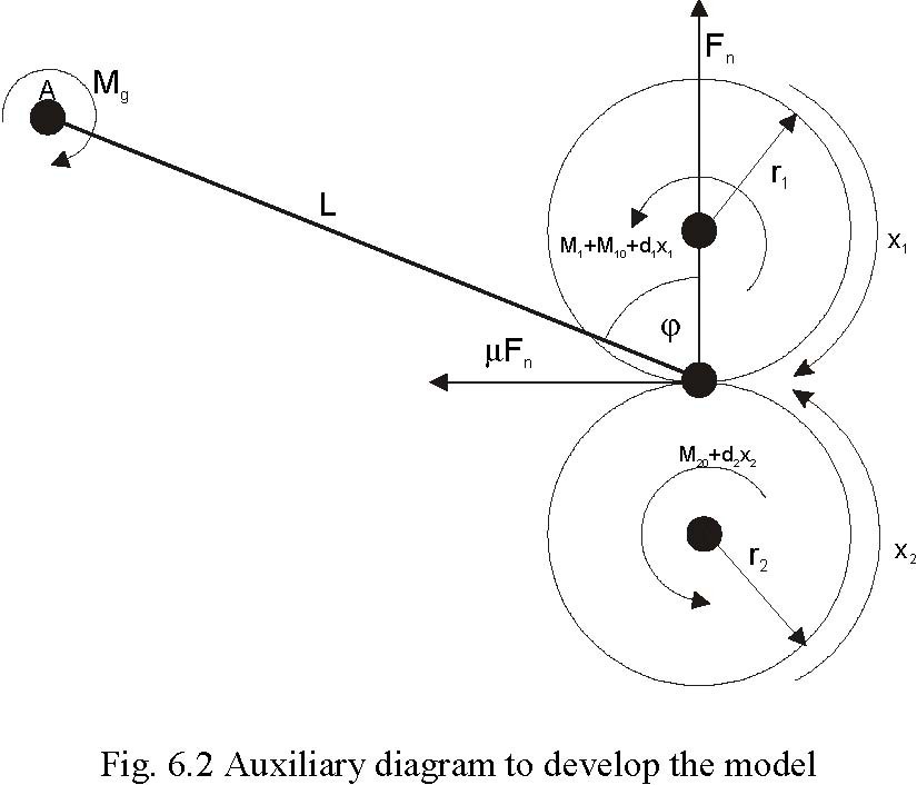
L
|
distance between the contact point of the wheels and the rotational axis of the balance lever (see Fig. 6.2)
|
m
|
|
ϕ
|
angle between the normal in the contact point and the line L
|
o
|
|
u
|
control of the brake
|
|
We assume that the friction force is proportional to the normal pressing force F . µ(λ) is the
n
proportionality coefficient. We introduce auxiliary variables:
s = sgn( rx − rx ) , (6.1)
22 11 s = sgn( x1) , (6.2)
1 s = sgn( x ) , (6.3)
22
We denote λ as the slip (the relative difference of the wheels velocities) in the following way
λ
=
À Œ Œ Œ Œ ŒŒÃŒ Œ Œ Œ Œ ŒÕ
rx − rx
22 11
, rx ≥ rx , x ≥ 0, x ≥ 0,
22111 2
rx
22
rx − rx
11 22
, rx < rx , x ≥ 0, x ≥ 0,
22111 2
rx
11
rx − rx
22 11
,
rx < rx , x < 0, x < 0,
22 111 2 (6.4)
rx
22
rx − rx
11 22
, rx ≥ rx , x < 0, x < 0,
22111 2
rx
11
1, x1 < 0, x2 ≥ 0, 1, x1 ≥ 0, x2 < 0.
6.1. Equations of motion
There are three torques acting on the upper wheel: the braking torque M1 , the friction torque in the upper bearing and the friction torque among the wheels. There are two torques acting on the lower wheel: the friction torque in the lower bearing and the friction torque among the wheels. Besides these we have two forces acting on the lower wheel: the gravity force of the upper wheel and the pressing force of the shock absorber.
We can write the following motion equation for the upper wheel Jx# = F rsµ(λ) − dx − sM − sM . (6.1.1)
11 n 1 11 110 11 We can write the following motion equation for the lower wheel Jx# =−Frsµ(λ) − dx − sM . (6.1.2)
22 n 2 22 220
To derive the normal force F we can write the sum of torques corresponding to the point A
n
(see Fig. 6.2).
FnL (sin ϕ− sµ(λ) cos ϕ) = Mg + s1M1 + s1M10 + d1x1 (6.1.3)
M + sM + sM + dx
g 11 110 11
F = . (6.1.4)
n
L(sin ϕ− sµ(λ)cos ϕ) Putting formula (6.1.4) to formulas (6.1.1) and (6.1.2) we obtain
M + sM + sM + dx
g 11 110 11
Jx# = rsµ(λ) − sM − dx − sM , (6.1.5)
11 1 11 11110
L(sin ϕ− sµ(λ)cos ϕ)
M + sM + sM + dx
g 11 110 11
Jx# =− rsµ(λ) − dx − sM . (6.1.6)
22 2 22220
L(sin ϕ− sµ(λ) cos ϕ) In both equations we have the common factor sµ(λ)
S(λ) =
L(sin φ− sµ(λ)cos φ)
. (6.1.7) µ(λ) can be approximated by the following formula
p
w4λ 32
µ(λ) =+ w λ+ w2λ+ w λ . (6.1.8) a +λp 31 It will be explained in Chapter 2 how to derive µ(λ) and S(λ) on the basis of experiments. We denote rd (sM + M )rd sMr 1
1 10 g 1
11 1 110 1
c = ,c = , c =− , c =− , c = ,c =− ,
11 12 13 14 15 16
J J JJJJ
1 1 1111
rd (sM + M )rdsM r
1 10 g 2
21 2220 2
c =− ,c =− , c =− , c =− , c =− .
21 22 23 24 25
J J JJJ
2 2 222 The equations (6.1.1) and (6.1.2) have the forms: x# = S(λ)(cx + c )+ cx + c +(cS(λ)+ c )sM , (6.1.9)
1 11 1 12 13 1 14 15 16 1 1 x# 2 = S(λ)(c21 x1 + c22 )+ c23 x2 + c24 + c25 S(x1, x2 )s1M1 , (6.1.10)
The driving system of the brake is described by the following equation
#
M1 = c (b(u) − M1) (6.1.11)
31
Constant is equal to 20.37 [1/s]. Function b(u) (see formula (6.1.11)) may be
c31 approximated by the formula:
b(u) =
ÀÃÕ
b
1
u + b ,u
2
≥
u
0
0,u < u
0
b = 15 .24 ,b = -6.21 ,u = 0.415.
120
6.2. Identification
6.2.1. Geometrical issues
At the beginning distance L, angleϕ and radiuses of the wheels (see Fig. 2) are measured. The following results are obtained (see Tab. 2.).
Table 2. Geometrical parameters
r1 r2 φ L
[m] [m] [°] [m]
0.0995 0.099 65.61 0.370
6.2.2. Deriving of torque Mg
From the formula (6.1.4) for x1 = 0 we obtain Mg = FnL sinϕ . Fnis measured by dynamometer or weighing conveyor (see Fig. 6.3)
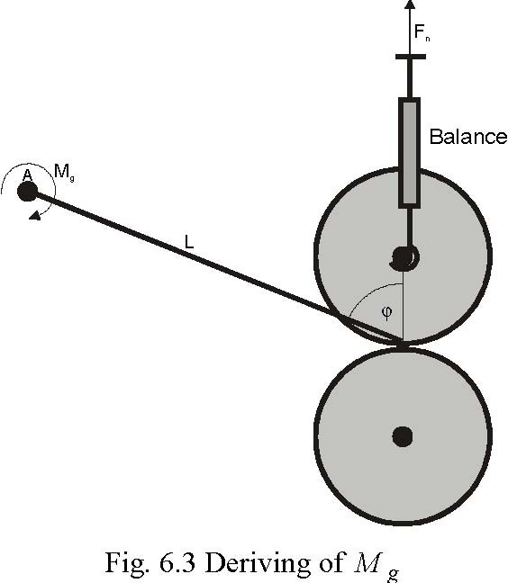
We obtain Fn = 58.214 N and we derive Mg = FnL sinϕ = 19.62 N.
6.2.3. Derivations of moments of inertia
J and J are derived on the basis of the upper and lower wheels velocities measured for a
12
constant driving torque applied to the considered wheel (see Fig. 6.4).

From formula (6.1) we obtain Jx# =−dx − M + mgr . (6.2.1)
11 1110 1
For a small x1 the first term of the right hand side can be neglected. Jx# =−M + mgr , x = 0. (6.2.2)
11 10 11(0) The solution of the above equation has the form mgr 1 − M10
x (t) = t . (6.2.3)
1
J
1 After few seconds the load is released and formula (2.3.1) becomes Jx# =−M , x (0) = x . (6.2.4)
11 10 1 10
M
x (t) = x − 10 t . (6.2.5)
110
J
1
mgr 1 − M10
The slope of line (6.2.3) is a1 = . Respectively the slope of line (6.2.5) is J1 − M10
a = .
J
1 Hence mgr 1 − M10 M10 mgr 1
a1 − a2 = += ,
J JJ
1 11 The moment of inertia is
mgr
1
J = .
1 a − a
12 The moment of inertia of the lower wheel is obtained. The results are given in Table 3. Table 3. Moments of inertia
|
J1 [kgm2]
|
J2 [kgm2]
|
|
7.53 10-3
|
25.60 10-3
|
6.2.4. Deriving the friction coefficients in the bearings
Viscous friction coefficients in the bearings and static frictions are derived on the basis of the following equations
Jx# =−dx − M
11 1110
Jx# =−dx − M .
22 2220
The coefficients are obtained by the mean square error method. Results are presented in Table 4 and Fig. 6.5.
Table 4. Measurement results of friction coefficients
|
|
Upper wheel
|
Lower wheel
|
|
d1 [kgm2/s]
|
M10 [Nm]
|
d2 [kgm2/s]
|
M 20 [Nm]
|
|
1
|
1.3436e-004
|
0.0022
|
2.1528e-004
|
0.0920
|
|
2
|
1.1978e-004
|
0.0025
|
2.1354e-004
|
0.0935
|
|
3
|
1.0209e-004
|
0.0050
|
2.1521e-004
|
0.0920
|
|
Mean value
|
1.1874e-004
|
0.0032
|
2.1468e-004
|
0.0925
|
Fig. 6.5 Experimental results. a), b) run of the upper wheel, c), d) run of the lower wheel. Blue – real time experiment, green – simulated model.
|
a) x [rad/s]
|
60 80 100 120 1
|
|
c)
|
80 100 120 140 160 180
|
|
|
0 20 40 0 20 40
|
60 80 100 120 t [s]
|
|
0 5 10 15 20 25 30 35 40 0 20 40 60
|
|
b)
|
0 20 40 0 20 40 60 80 100 120 x 1[rad/s]
|
60 80 100 120 t [s]
|
d)
|
0 5 10 15 20 25 30 35 20 40 60 80 100 120 140 160 180 t [s] x 1 [rad/s]
|
6.2.5. Identification of the friction coefficient and the braking torque
From formulas (6.1) and (6.2) we have
» r ÿ
2
M1 =−… (J 2 x# 2 + d2 x2 + M 20 )+ J1x#1 + d1x1 + M10 Ÿ (6.2.6) r1 ⁄ The braking torque versus velocity x1 and control u is derived from formula (6.2.6). From formulas (6.1.2) and (6.1.4) we obtain
Mg + M1 + M10 + d1x1 Jx# + dx + M
2222 20
F = =− . (6.2.7)
n
L(sin φ−µ(λ)cos φ) ()
µλ r2
Lsinφ
(Jx# + dx + M )
2222 20
r
µ= 2 (6.2.8)≈ L cosφ r2 ’
(J 2 x# 2 + d2 x2 + M 20 )ΔΔ + ÷÷ + J1x#1 − Mg « r2 r1 ◊
From formula (6.2.8) the friction coefficient versus the slip is calculated. The accelerations in formulas (6.2.6) and (6.2.7) are not measured. They are observed on the basis of the measured velocities.
A number of experiments have been performed. In every experiment the wheels are accelerated to reach the angular velocity about 180 rad/s. Next, the brake procedure begins. The small DC motor responsible for braking obtains jump of control of magnitude between 0 and
1. The wheel velocities are registered during the brake procedure. On the basis of formulas
(6.2.6) and (6.2.7) the mean square braking torque and the friction coefficient corresponding to the upper wheel is derived. The results of experiments are presented in Fig. 6.6
approximated by the formula:
b(u) =
15.24 u -6.21, u
ÀÃÕ
≥
0.415
0.12, u < 0.415
The model coefficients have the following values:
= 0.00158605757097, = 2.593351896228796e+002,
c11 c12
== 0.01594027709515, = 0.39850692737875,
c11 c13 c14
= 13.21714642472868, = 132.8356424595848,
c15 c16
= 0.000464008124048, = 75.86965129086435,
c21 c22
= 0.00878803265242, = 3.63238682966840,
c23 c24
= 3.86673436706636, = 20.37,
c25 c31 w1 =− 0.04240011450454, w2 = 0.00000000029375, w3 = 0.03508217905067, w4 = 0.40662691102315 a = 0.00025724985785, p = 2.09945271667129.
7. Simulation of braking
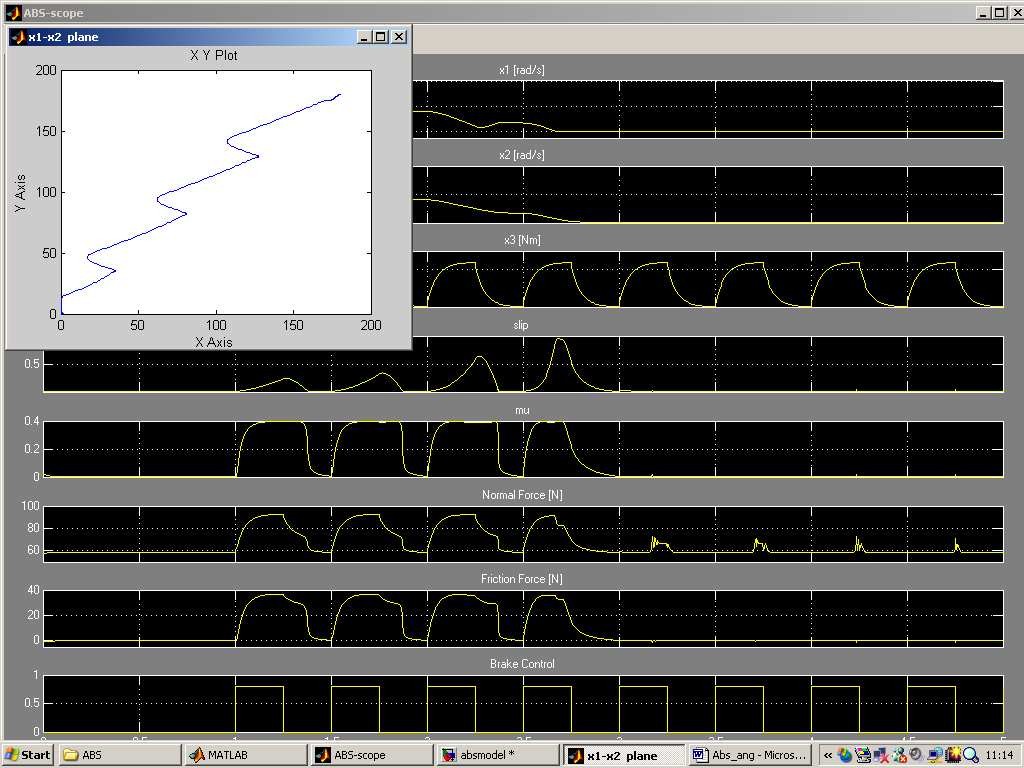
The ABS dynamical model has been created in Simulink (see the green box in Fig. 7.1)
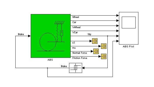
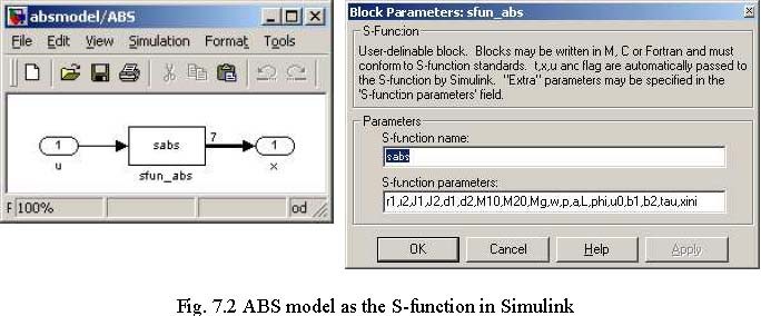
The ABS block has one input u and nine outputs x. The brake control is the input variable. The output variables are visible in Fig. 7.1. These are: Wheel, Car, VWheel = x1, VCar = x , Slip =λ, M = x , mu =µ, Normal Force = F , Friction Force =µ F . In
2 13 nnfact, the model is the S-function denoted sfun_abs (see Fig. 7.2). We can see the interior obtained after looking under mask (the left hand side picture) and the parameters of the S-function (the right hand side picture). A user can define 19 parameters of the S-function from
to .
r1 xini
If one clicks on the green box the following mask appears (see Fig. 7.3).

We can perform the simulation of the model corresponding to the parameters given in the mask. The following graphical data are obtained in ABS scope and x1-x2 plane (see Fig. 7.4).
The X Y Plot shows the state variables x1 vs. x2 . In the ABS scope one can see time responses of different variables related to the input brake control (the last diagram). We can verify the accuracy of the model investigating how close these responses are to the real system responses.
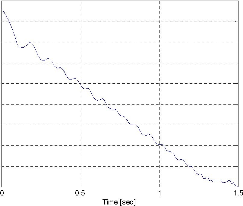
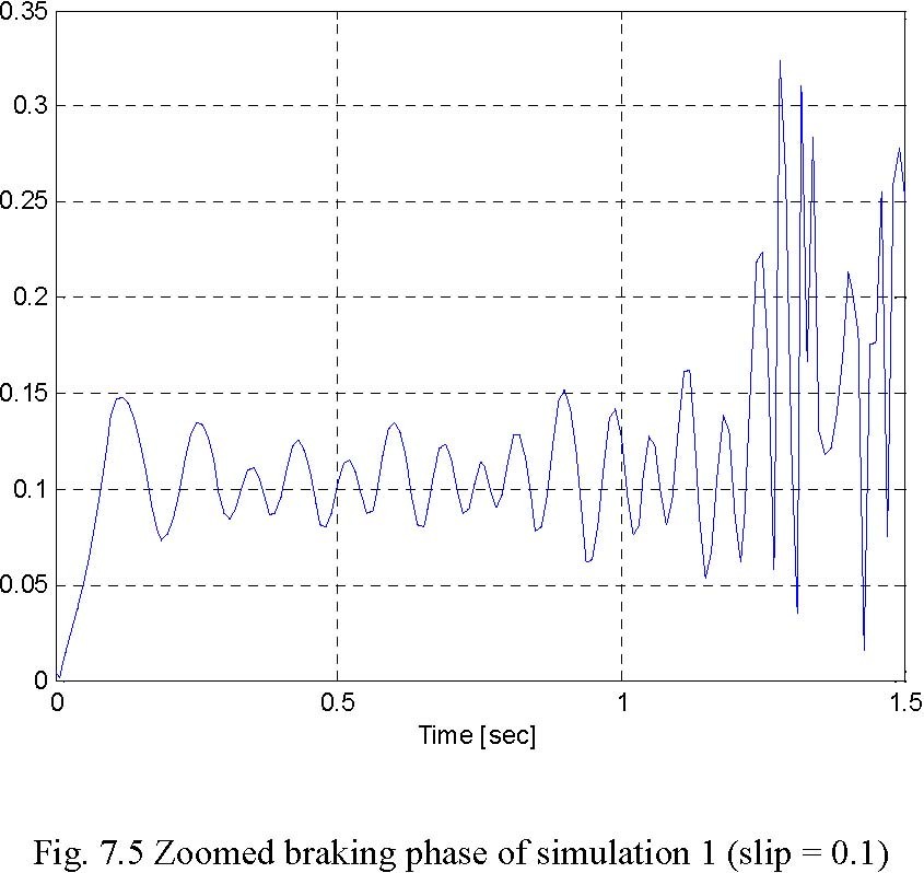
Using the model given in Fig. 7.1 with a relay feedback we obtain simulation results. We perform simulation 1 identical to the experiment 1 (see Fig. 4.11). In this experiment the slip defined in the relay block is equal to 0.1. We simulate only the braking phase. Therefore the initial car velocity is assumed to be equal to 1800 rpm. The zoomed braking phase of simulation 1 is given in Fig. 7.5. One can notice the similar braking time (approx. 1.5 seconds) in both: real-time experiment 1 (Fig. 4.11) and simulation 1 (Fig. 7.5). The experimental and simulated slips correspond also one to another. Simulation 2 is performed for the slip defined in the relay block equal to 0.7. The zoomed braking phase of simulation 2 is given in Fig. 7.6. We can notice similarities between the real-time experiment 2 (see Fig. 4.13) and simulation 2 (see Fig. 7.6). As in the first example we simulate only the braking phase of control. In fact a slip cannot be negative. This is guaranteed due to formula (6.4). However the slips in the real-time experiments calculated from the velocities obtain negative values. We must remember that the car and wheel velocities are not measured. They are only observed. Large velocity errors are introduced if the velocities bring low values.
Car velocity [rpm] (braking time)
1800 1600 1400 1200 1000 800 600 400 200 0
Slip 0.1 (braking time)
Time [sec] Car velocity [rpm] (braking time)
1800 1600 1400 1200 1000
800
600
400
200
0
-200

0 0.5 1 1.5 Time [sec]
Slip 0.7 (braking time)

Time [sec]
inteco  收藏灵猫网
收藏灵猫网